BACKGROUND · OVERVIEW · PARAMETERS · CLASS METHODS · EXAMPLE USGAE · CONCLUSION · GITHUB
BACKGROUND
One of my hobbies is designing and creating yarn crafts, I wanted to use C2C technique in crochet to make blankets and needed a reliable (and free) way of creating pixelated images and group/cluster the colors in the image to a reasonable number (it would be awfully difficult to make a blanket with 200 different shades of each color 😆). So I figured why not write a Python code to do exactly this! All code and example usgage can be seen in my GitHub repo.
The pixelation process is written in vanilla Python, while K-Means clustering is used to group the colors. All work was done in Google Colab (Free). Notable Python packages used:
- standard: numpy, pandas
- image processing: PIL Image
- modeling: scikit-learn
- visualization: matplotlib
- parameter validation: pydantic
OVERVIEW
The entire algorithm is wrapped in one class called Processed. When I first wrote the code, I first wrote the steps outside of functions, then I wrapped the steps in functions for better visibility and at the end wrapped all functions within the one class. The class accepts six parameters as inputs, Pydantic is used to validate the parameters (see ProcessImageInput class). The contains n supporting methods in addition to __init__() to process the image based on the specified parameters.
PARAMETERS
The six supported parameters are as follows.
- input_image_path: str
- Path to the input image file.
- Called by the _process_image() function within the class to load the image from the specified path.
- resize_ratio: float
- The ratio by which the image should be resized. Default=0.1
- Called by the resize_image() function within the class to resize the image.
- Only positive values are accepted.
- Values between 0 and 1 decrease the image size while values > 1 increase the image size.
- Images are sized to proportion of the original image.
- grid_size: int
- The size of the grid for pixelation. Default=10
- Called by the resize_image() function within the class to adjust the size the image to be divisible by the grid size to prepare for pixelation.
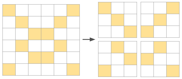
- Called by the image_pixelates() function within the class to pixelate the image based on the specified size. Below is a visualization of what the grid_size represents.
- Only positive values are accepted.
- Images can be viewed as representations of little boxes (ie, pixels). See below example, if our image is of size (6x6), a grid_size=3 would cover each of the (3x3) grid within the image, the grids are non-overlapping. Our (6x6) image can then be represented with four (3x3) grids.
- do_reduce: bool
- Flag indicating whether to reduce the number of colors using k-means clustering. Default=False
- cluster_metric: str
- Method for identifying number of clusters. Default='ch'
- Ignored if do_reduce == False.
- Acceptable inputs are as follows. The spelling of the input has to be exact as the supporting functions for the methods are dynamically called based on the string passed in.
- 'sil': silhouette method
- 'db': davies bouldin method
- 'ch': calinski harabasz method
- Another commonly used technique for identifying optimal number of clusters is by using the Elbow method of visually inspect the number of clusters and the respective WCSS value for that cluster. As this method requires visual inspection, it is not as systematic as the other methods, so I did not implement this method in the algorithm.
- num_colors: int
- Maximum number of colors/clusters to reduce to. Default=12
- Ignored if do_reduce == False.
- Must be >= 2.
- Called by each of the cluster_metric() function to determine the optimal number of clusters.
CLASS METHODS
The __init__ method instantiates the Processed class. Once the parameters have been initiated, the _process_image() method is called to begin processing the image.
The 9 supporting methods are as follows.
- _process_image():
- Process the input image based on the specified parameters.
- A 'private' method within the class that's called when the class is instantiated.
- Loads the image from the input_image_path, calls the resize_image() method to resize the image, calls the image_pixelates() method to pixelate the resized image, then calls the display_pixelated_image() method if the flag for do_reduce is set to False, or calls subsequent clustering methods if the flag for do_reduce is set to True.
- resize_image():
- Resize the given image based on the specified ratio and grid size.
- Takes in the loaded image, resize_ratio, and grid_size as parameters.
- Returns the resized image to _process_image() method to be used in subsequent methods.
- First adjusts the new dimensions to ensure the width and height are divisible by the grid_size, then uses the PIL Image built in method .resize() to resize the original image to the new dimensions.
- get_pixelates():
- Pixelate the given image into a grid of the specified size.
- Takes in the loaded image and grid_size as parameters.
- Iterate over the columns and rows of the image, use the PIL Image built in method .crop() to crop the image based on specified grid size, store the cropped image in a dictionary with the key being the column index and the values being a list of cropped images for each column index.
- display_pixelated_image():
- Displays the pixelated image.
- Takes in the image, grid_size, and the cropped images from get_pixelates() as parameters.
- For each cropped image of size == grid_size, find the predominant_color of that grid and represent that grid with only the predominant_color.
- get_predominant():
- Get the predominant colors of all grids.
- Takes in the image, and the cropped images from get_pixelates() as parameters.
- Similar to display_pixelated_image() method, except this method returns the predominant colors in the form of a list, whereas the display_pixelated_image() method directly displays the image.
- xxx_method():
- Three methods used to find the optimal number of clusters based on the method specified when instantiating the class.
- Dynamically called by the _process_image() method and returns the optimal number of clusters based on the selected method.
- Take in the maximum number of clusters and the predominant_colors (as returned by the get_predominant() method) as parameters.
- get_centroids():
- After finding the optimal number of clusters, find the centroids using k-means clustering.
- Takes in the optimal number of clusters (as returned by the xxx_method() method) and the predominant_colors (as returned by the get_predominant() method) as parameters.
- Returns the centroids and display the centroid colors.
- get_predominant_color_mapping():
- After finding the centroids, map each predominant color to its nearest centroid.
- Takes in the centroids (as returned by the get_centroids() method) and the predominant_colors (as returned by the get_predominant() method) as parameters.
- Returns the predominant_color_mapping in the form of a dictionary, with the predominant color as the key and the centroid as the value.
- display_reduced_colors_image():
- Similar to display_pixelated_image(), but instead of directly displaying each grid as the predominant color for that grid, display the centroid mapped to the predominant color for the grid. By using centroids instead of predominant colors, the number of colors in the overall image is reduced to the number of centroids.
- Experiments should be conducted to identify the best hyperparameters to represent the image while preserving the image integrity.
EXAMPLE USAGE
Below is a sample code chunk to initiate the inputs, ProcessImageInput() is a Pydantic BaseModel class used to validate the inputs. The input_image_path parameter is required while the other parameters are optional. If the other parameters are not passed in, the default values will be used. See the parameters section for the default values. Extra parameters are prohibited.
      input_params = ProcessImageInput(input_image_path="your/path/cat.jpeg",
                                       resize_ratio=1.1,
                                       grid_size=5,
                                       do_reduce=True,
                                       cluster_metric='db',
                                       num_colors=5)
Once the inputs are validated, the Processed class can be instantiated by passing in the input parameters, the _process_image() method is automatically called when the class is instantiated. The image is automatically processed based on the parameters.
processed = Processed(input_params)
The class variables can be extracted, and the 'public' class methods can be called by passing in the required parameters.
      # get the centroids as processed
      new_centroids = processed.centroids

      # manually replace the centroids to desired colors based on visual inspection of the centroid
      new_centroids[0] = [0,0,0] # black
      new_centroids[1] = [102,51,0] # brown
      new_centroids[2] = [210,180,140] # tan
      new_centroids[3] = [255,0,0] # red
      new_centroids[4] = [255,0,0] # red

      # display the image with the new centroids
      processed.display_reduced_colors_image(processed.resized_image,
                                             processed.grid_size,
                                             processed.image_pixelates,
                                             processed.predominant_color_mapping,
                                             new_centroids)
Cat
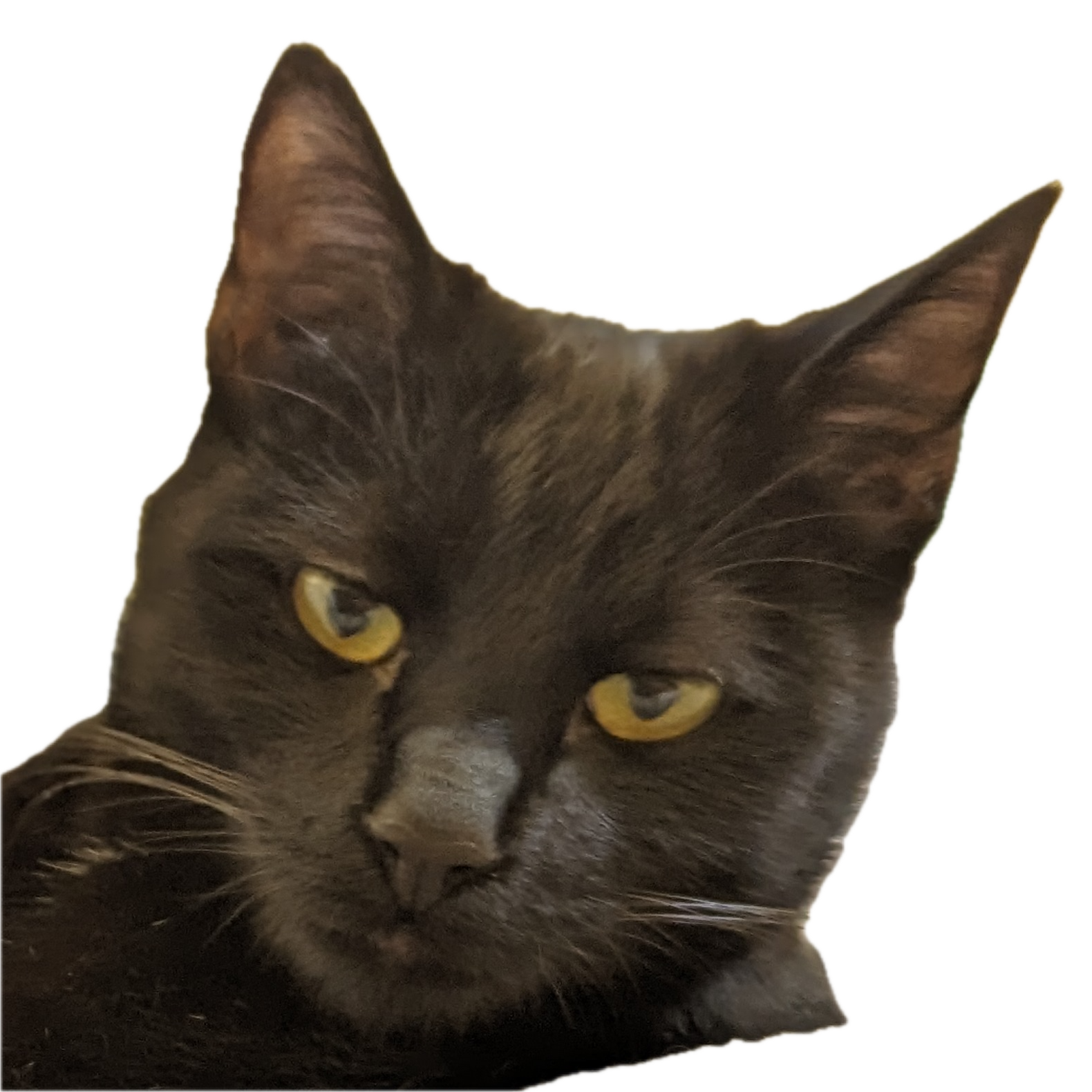
For experimentation, I found an image of a cat from Google, first rendered the pixelated image without clustering, with resize_ratio=1.1 and grid_size=5, then rendered the pixelated image with the three different methods of clustering (each with the same num_colors=12), while holding the other parameters constant. Below is a comparison of the images at different stages.
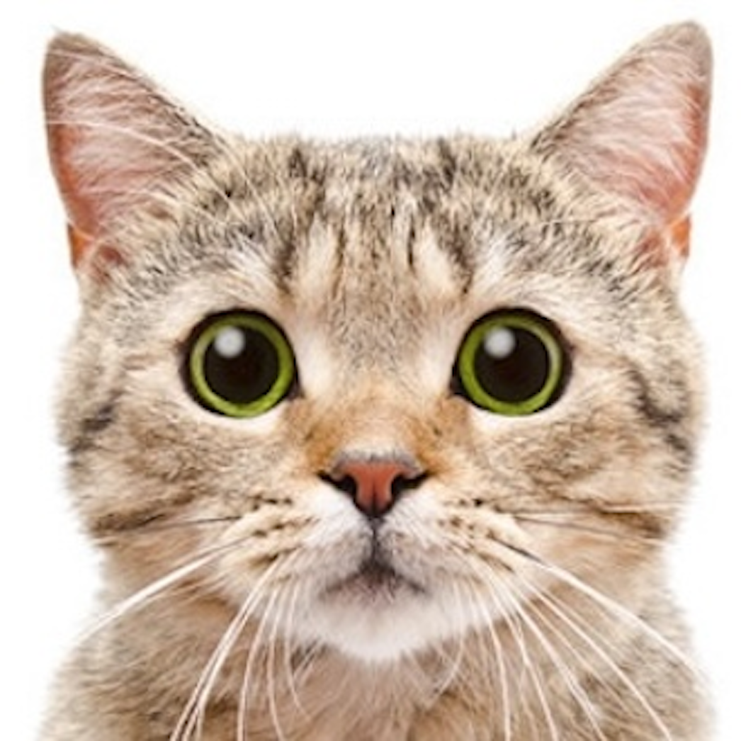
original cat image
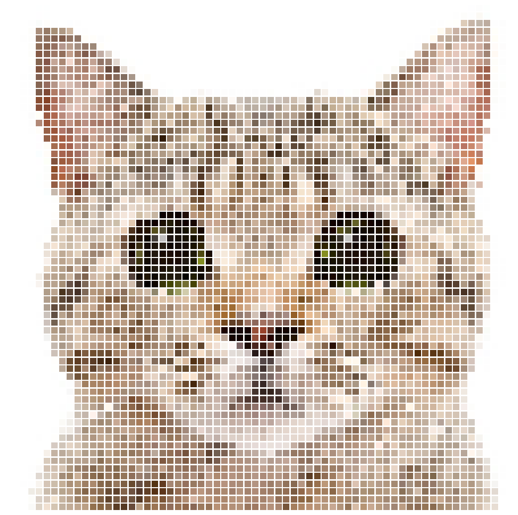
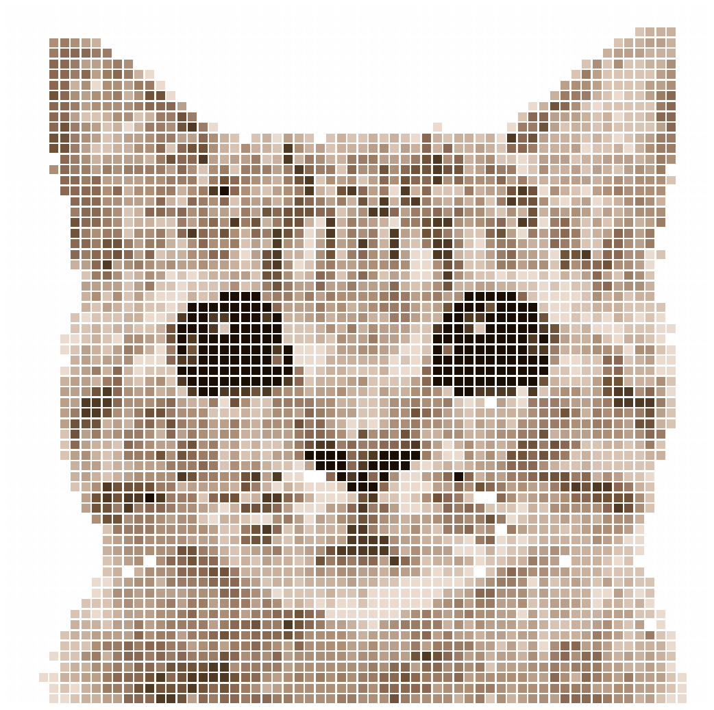
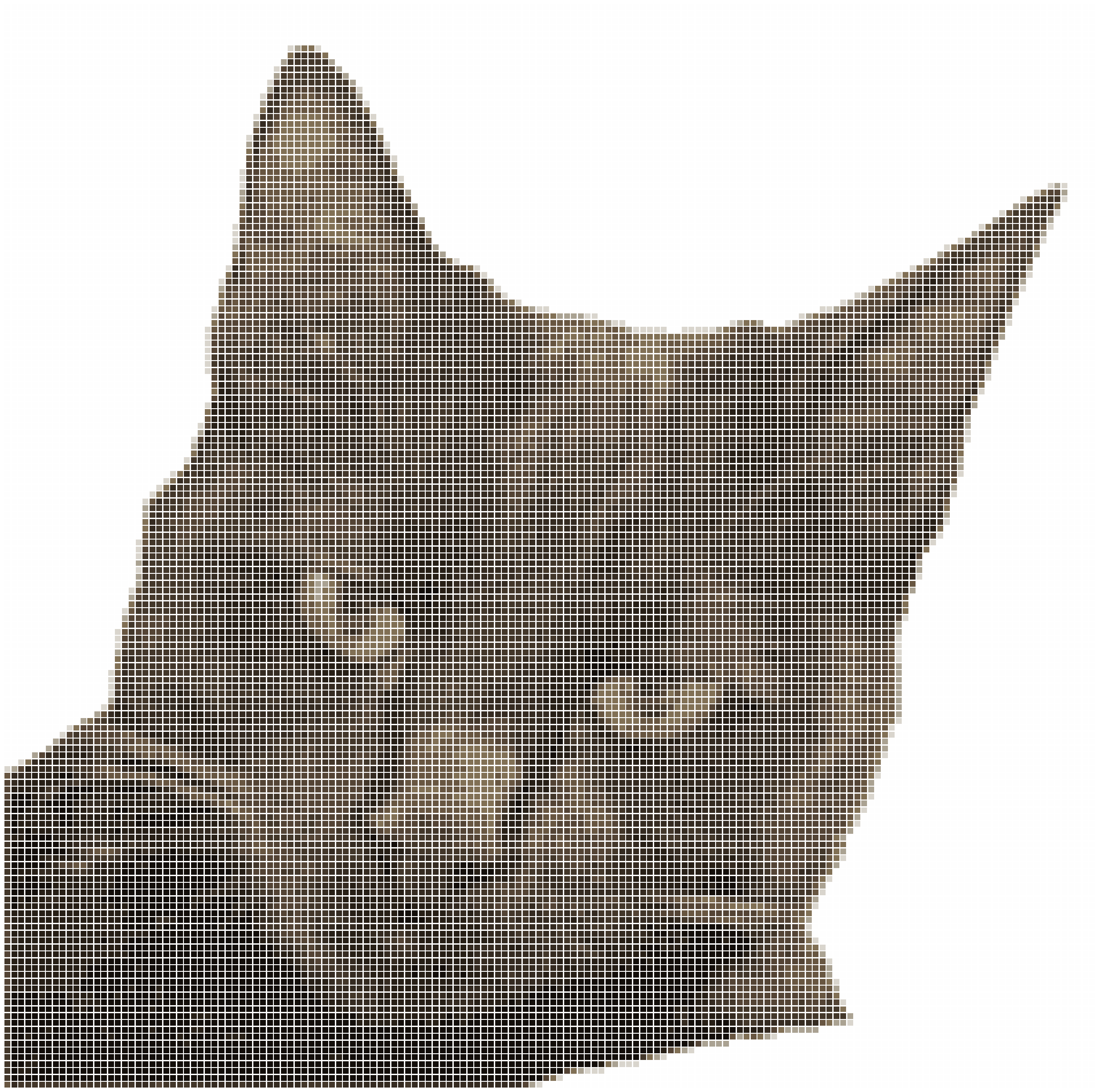
pixelated cat without clustering
The pixelated without clustering image is a surprisingly good representation of the original image, we can even still see the green eyes and the pink nose.

pixelated cat with sil clustering
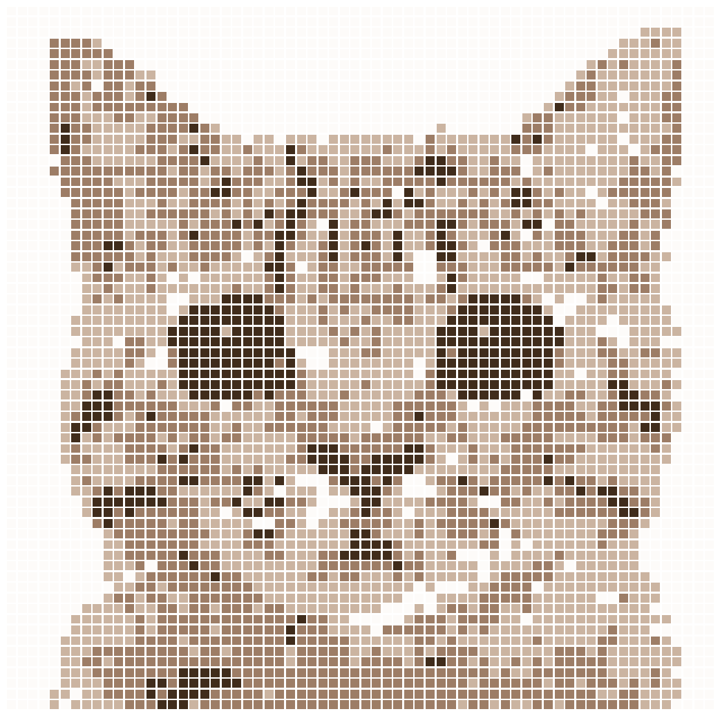
pixelated cat with db clustering
pixelated cat with ch clustering
Both sil and db methods found the optimal number of clusters == 4, where as the ch_method found 11 (with 12 being the maximum number of clusters as passed in the parameters). I would argue even with only 4 colors, the pixelated image is till a pretty decent representation of the original image, but since the background of the image is white, some lighter colored pixels in the image are replaced with white when the number of clusters == 4, which I did not like. The green eyes and the pink nose are also now replaced with generic brown colors after clustering.
Tofu
Since the previous image contained only plain background with mostly brown colors, I wanted to try an image with more colors and with a busy background. So I used an image of our dog Tofu wrapped in a blanket. I went straight to with clustering this time, since the main goal of this project is color reduction. The original image size was reduced by setting resize_ratio=0.2 and I used grid_size=8.
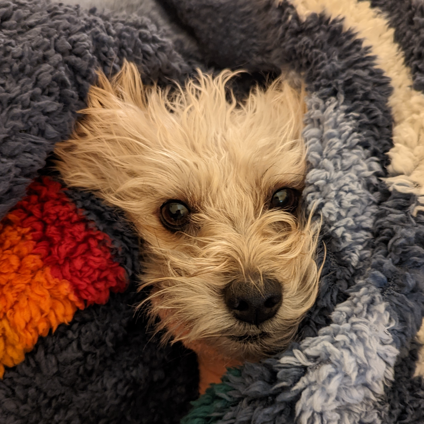
original Tofu image
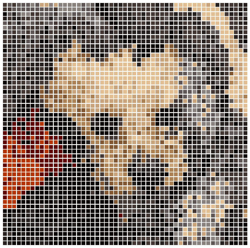
pixelated Tofu with ch clustering
Similar to the previous experiment, both sil and db methods reduced the number of colors drastically, in this case, the number of colors were reduce to only 2 (which is the minimum as defined in the class). The ch method image is better, but really not that great, the finer details of her face is no longer visible, this might be attributable to a larger grid_size as more pixels are now been combined together to one grid.

pixelated Tofu with sil clustering
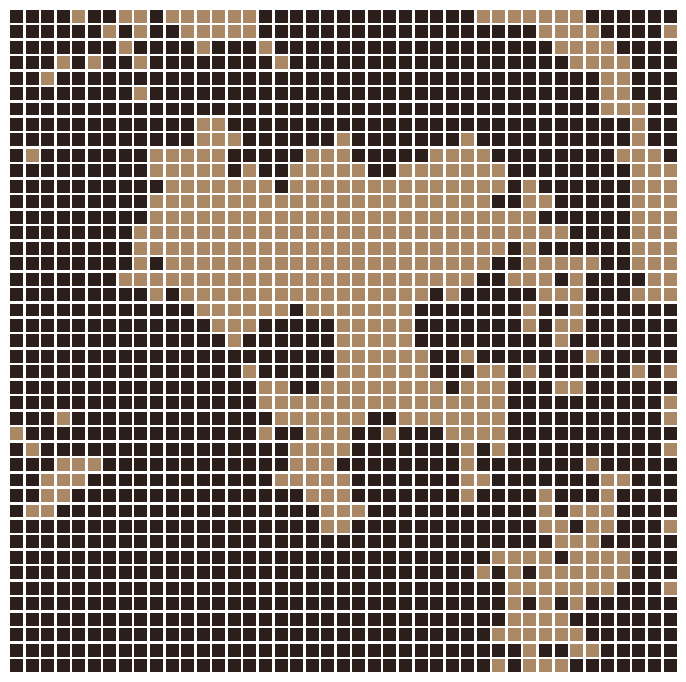
pixelated Tofu with db clustering
Tux
I am now curious to see how the pixelation would turn out if the grid_size is set to 1, meaning the pixels in the original image are retained and not aggregated to grids. For this experiment, I used an image of our cat Tux, he is a black cat so I figured the algorithm might struggle since we often struggle with even taking clear photos and videos of him as the camera keeps going out of focus because of his fur. I used an image editor tool to remove the background from the original image and reduced the original image size by setting resize_ratio=0.1.
original Tux image
pixelated Tux with ch clustering
I knew there was probably no point in trying the sil and db methods since these two methods seem to tend to reduce the number of clusters drastically, so I went ahead with the ch method with maximum number of clusters set to 12. The algorithm selected 10 centroids and the rendered pixelated image is actually pretty good, his facial features are still clearly visible, as well as his yellow eyes.
Miata
Since I've only experimented with animals so far, I figured I should try something different next. So I used an image of our Miata, a happy little car that we love (if you don't have one, you should!). I reduced the original image size by passing in resize_ratio=0.1 and used grid_size=5.
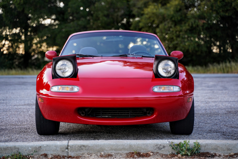
original Miata image
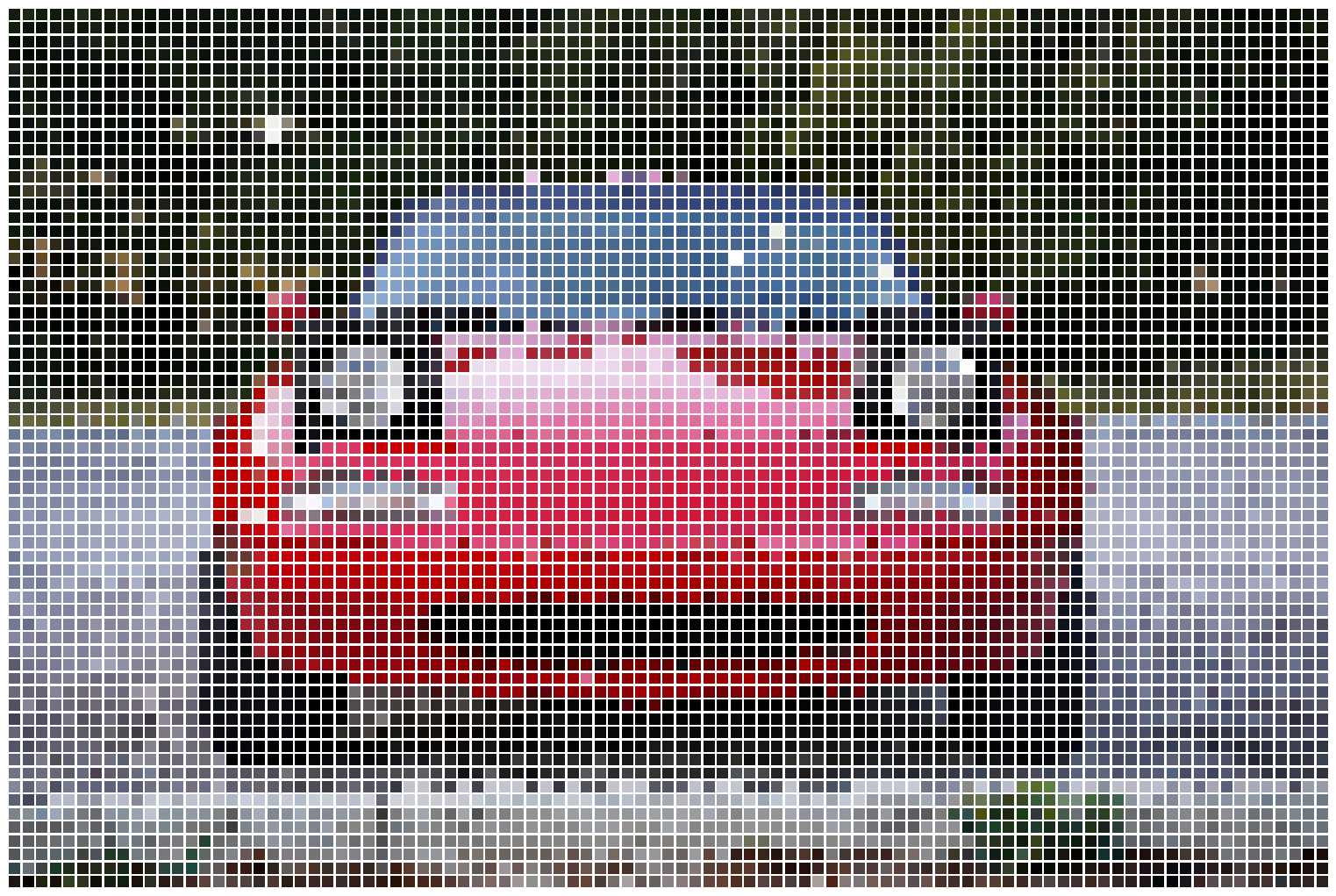
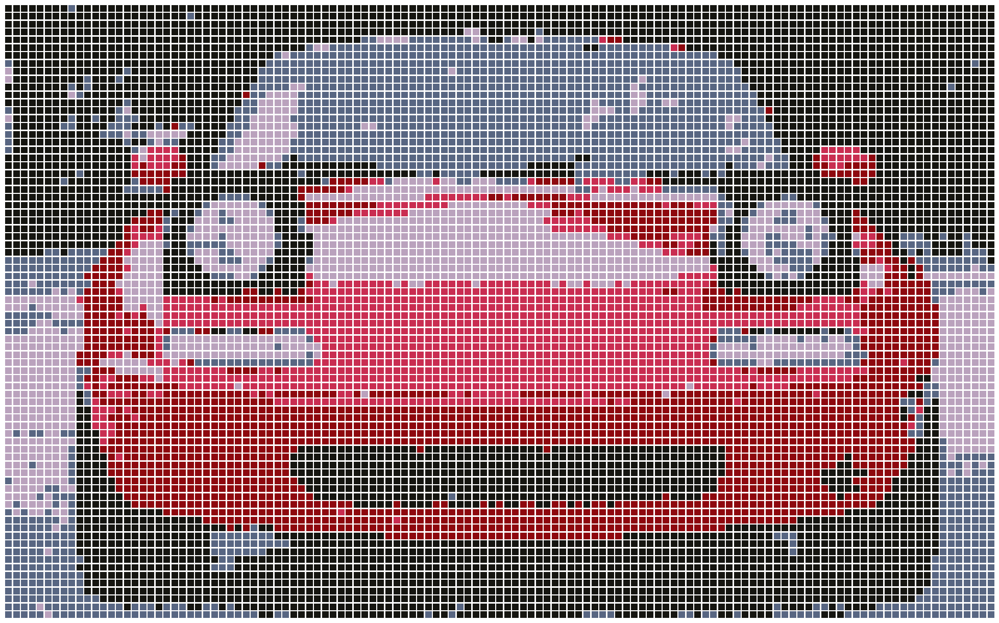
pixelated Miata without clustering
The pixelated without clustering image is again a very good representation of the original image, we can still see some of the trees in the background and the curb at the front.

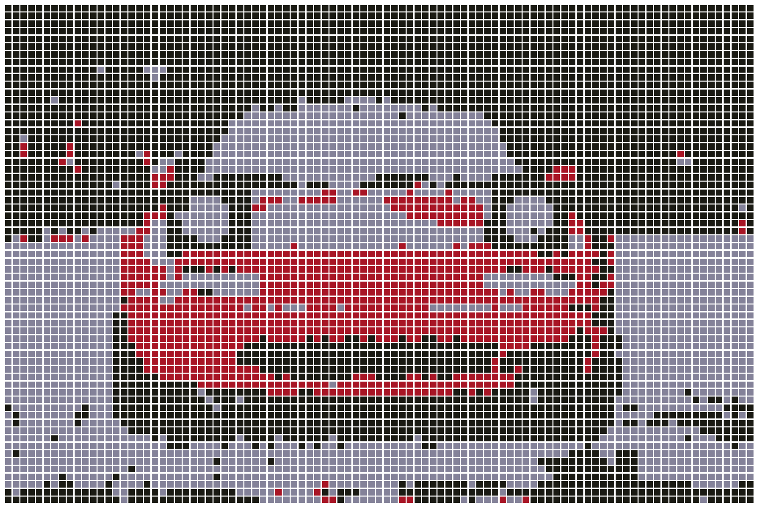
pixelated Miata with sil clustering
pixelated Miata with db clustering
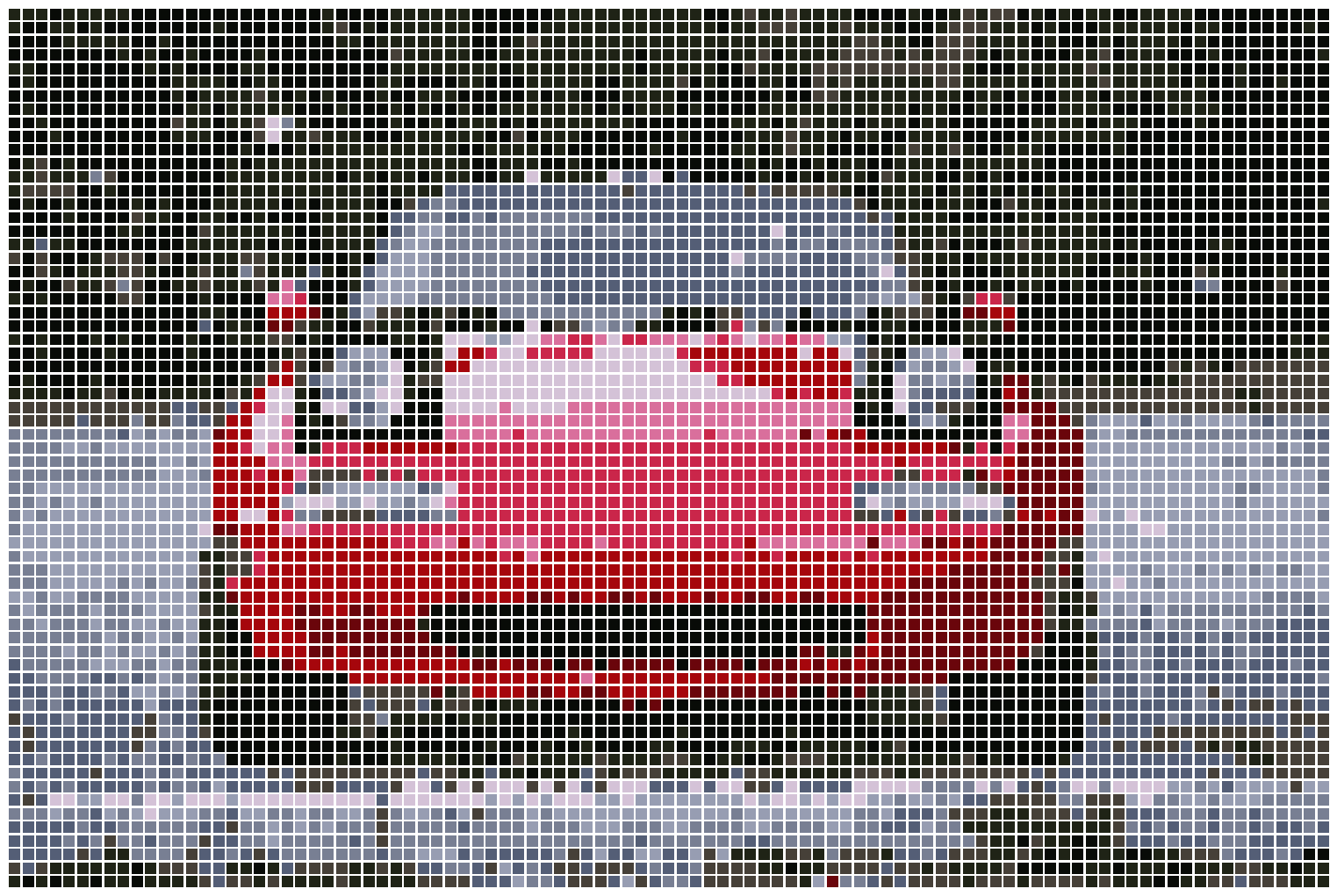
pixelated Miata with ch clustering
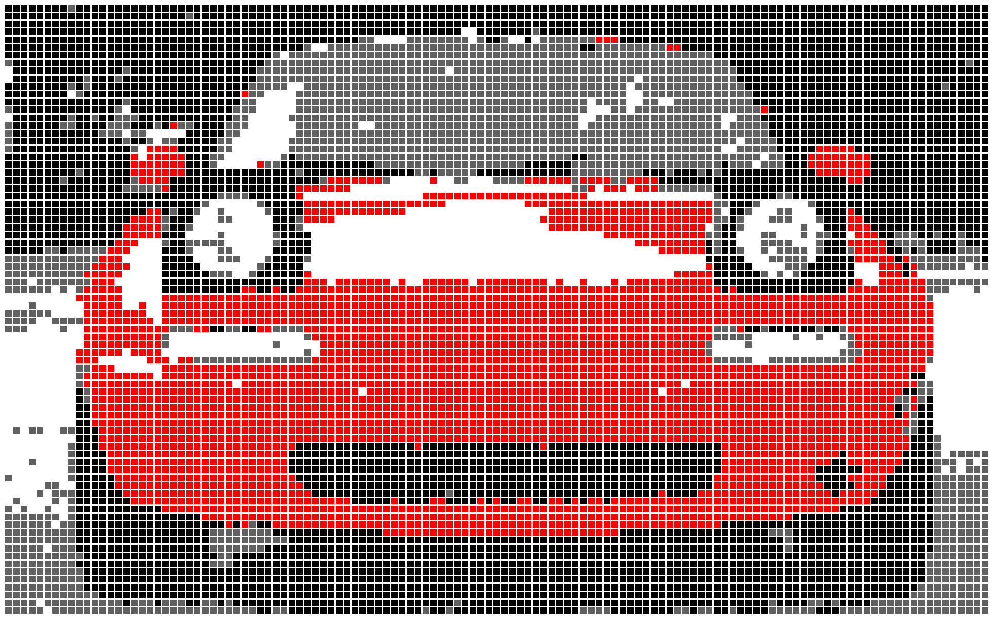
Similar to the previous experiments, both db and sil methods reduced the number of colors drastically (only 3 colors), while the ch method reduced the number of colors to 11. Even with only 3 colors, the car is still clearly visible, although there is now more noise in the background as some of the green colors in the background is now replaced with red (interesting), and the reflection on the hood is not as crisp. The one with ch method is certainly a better representation, but in all of them, the red roof is now no longer visible, perhaps this could be improved by reducing the grid_size. Also I feel 11 colors is still too many colors, since we can see that the image was rendered decently well with only 3 colors, so perhaps we could reduce the number of clusters.
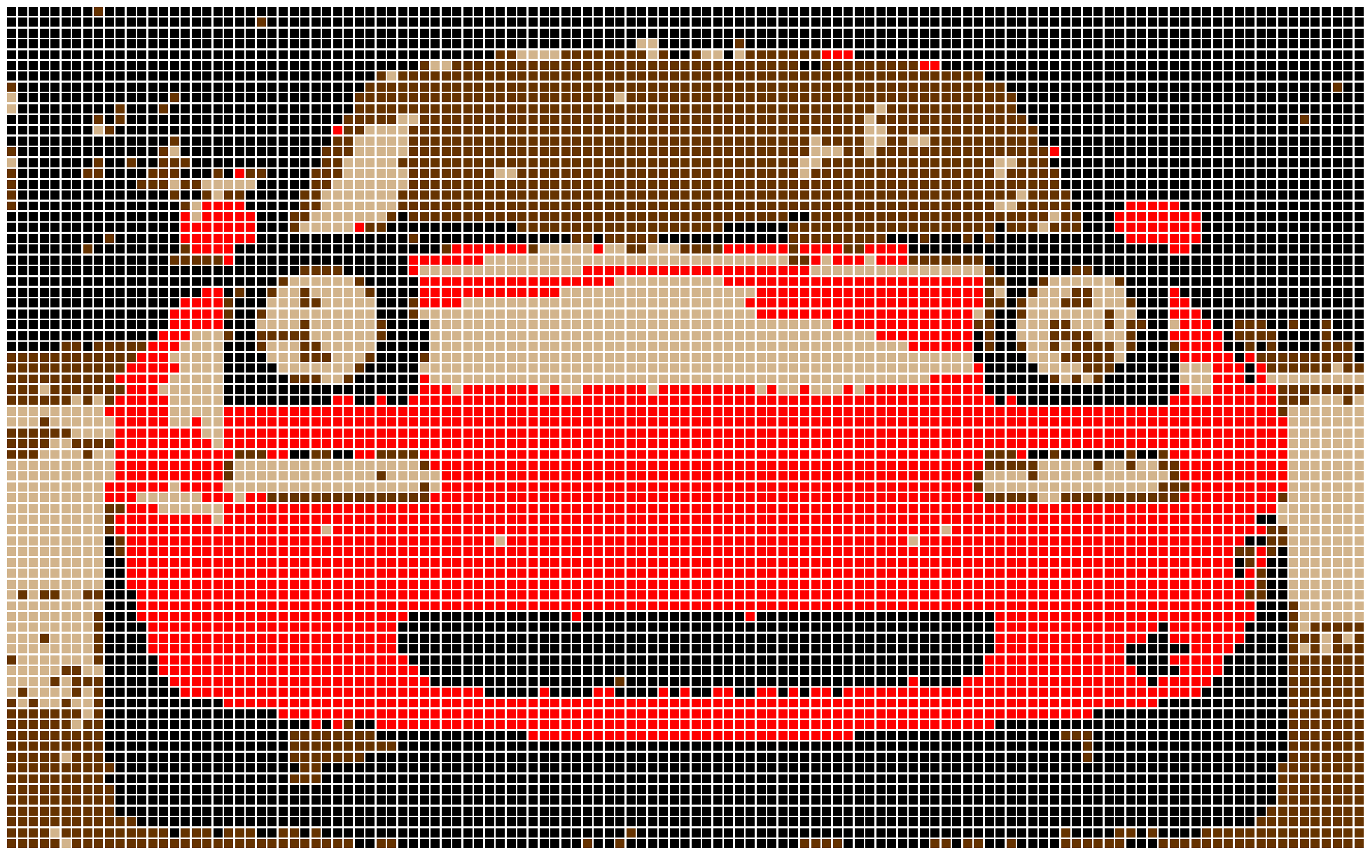
So I then tried reducing the grid_size to 3 and reducing the maximum number of clusters to 7, with ch method, which reduced the optimal number of clusters to 5, with below 5 colors as the centroids. This is now looking really amazing! I love how the Miata came out, and the colors adds a 'retro' look to the image, which fits the car just perfectly!
pixelated Miata with ch clustering and 5 centroids

centroids
But remember I mentioned that I started this project because I wanted to create a way to make pixelated images for crocheting blankets? Since I did not have the yarn colors that match the centroids, I needed to replace some of the centroid colors with the yarn colors that I had. Here are two versions based on the yarn colors I had at hand. I combined the two redish colors to red and replaced the greyish blue color and the light purple color respectively. The manually adjusted versions are certainly not as nice as the originally rendered version, but the one with white and grey (the one on the right) actually turned out looking decent. I am still working on the blanket at the time of writing, but I'll be sure to show you the finished blanket when it's done! The code used to manually adjust the centroid colors can be found in the 'miata.ipynb' notebook on the GitHub.
pixelated Miata with manually adjusted centroids
pixelated Miata with manually adjusted centroids

centroids

centroids
CONCLUSION
That's it for this project, I had a lot of fun working on it and will certainly be using the code in my crochet projects. The code could definitely be optimized, especially since the code is currently processing the grids sequentially, but perhaps there is a way to better parallelize the process, which I will work on next!
GITHUB
Please see my GitHub for the code for the project.