DESCRIPTION · BACKGROUND · MOTIVATION · DATA SOURCE · DATA CLEANING · EDA · MODEL · LIMITATIONS · GITHUB · MEMBER CONTRIBUTIONS
DESCRIPTION
This project utilized Large Sample Ordinary Least Squares (OLS) Regression to evaluate the possible causal relationships between Body Mass Index (BMI) and cholesterol ratio. Data was sourced from the 2005-2006 National Health and Nutrition Examination Survey (NHANES), and all data cleaning, analysis, and model building were conducted using the R programming language.
BACKGROUND
This was the final project for the Statistics for Data Science class in my Masters in Data Science program, a collaborative effort involving me and three other classmates.
The objective was to formulate a research question that distinctly identifies an independent variable (X), representing a modifiable 'product feature' and a dependent variable (Y), representing a 'metric of success'. The interpretation of 'product feature' and 'metric of success' was broad and extended beyond tangible products and sales.
Guided by the project requirements, we utilized R as our programming language and conducted an explanatory study using Ordinary Least Squares (OLS) regression. While OLS regression might not be the most appropriate approach to establish causal relationships with observational data, the assignment emphasized constructing a model that is reasonably plausible.
All work was done in RStudio, with R as the programming language. Notable R packages used:
- general: tidyverse/dplyr
- modeling: effsize, car, lmtest, sandwich
- visualization: ggplot2, stargazer, knitr
MOTIVATION

nearly 1 in 3 adults are overweight

more than 2 in 5 adults are obese
The increasing prevalence of obesity and its associated health complications has become a public health concern. One of the most significant health risks associated with obesity is elevated cholesterol levels, a leading risk factor for cardiovascular diseases such as heart attacks and strokes.
With this motivation in mind, we proposed the research question:
Does a higher BMI cause a higher cholesterol ratio?
where our 'product feature' is weight health, operationalized using Body Mass Index (BMI), calculated as weight in kilograms divided by height in meters squared, and our 'metric of success' is cholesterol, operationalized using cholesterol ratio, calculated as total cholesterol divided by HDL. We considered the use of total cholesterol or other cholesterol measurements but ultimately decided on the cholesterol ratio, the reasoning can be found in the final report.
DATA SOURCE
The project guideline specified that the data must be cross-sectional with a minimum of 200 observations, and the dependent variable must be metric. An example of non-cross-sectional or longitudinal data is time series, where the value from the previous day directly impacts the next day. Cross-sectional data is required to minimize the possible independence violation in the independent variables. An example of non-metric or ordinal data is the Likert scale, ordered categorical data, where the distance between each category is unknown.
With the project guideline in mind, we obtained the data from the 2005-2006 National Health and Nutrition Examination Survey (NHANES). The NHANES conducts annual surveys of individuals across the United States, and the 2005-2006 survey selected 10,348 individuals for the sample. The dataset contains separate files for demographics and results from each examination, laboratory, and questionnaire. Each row of the files represents a unique individual identifiable by a unique sequence number.
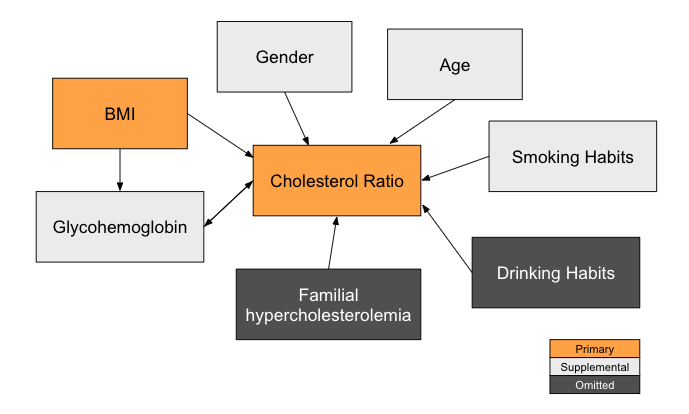
With cholesterol ratio as our dependent variable and BMI as our primary independent variable, we also considered additional covariates that could impact the dependent variable. Some supplemental independent variables we included in our models are glycohemoglobin (a lab test that measures the average level of blood sugar in an individual), age, gender, and smoking habits. Due to the lack of sufficient data in our dataset, several omitted variables are excluded in our models, such as drinking habits and familial hypercholesterolemia (a genetic disorder that has a strong relationship with high cholesterol).
Below is a causal diagram to visualize the various variables in the model.
Primary Variables
| Dataset | Variable Name | Variable Description | User Guide |
|---|---|---|---|
| DS13 Examination: Body Measurements | SEQN | Respondent sequence number | Page 10/129 |
| BMXBMI | Body Mass Index (kg/m**2) | Page 15/129 | |
| DS129 Laboratory: Total Cholesterol | SEQN | Respondent sequence number | Page 8/65 |
| LBXTC | Total cholesterol (mg/dL) | Page 8/65 | |
| DS111 Laboratory: HDL Cholesterol | SEQN | Respondent sequence number | Page 10/67 |
| LBDHDD | Direct HDL-Cholesterol (mg/dL) | Page 10/67 |
Supplemental Variables
| Dataset | Variable Name | Variable Description | User Guide |
|---|---|---|---|
| DS110 Laboratory: Glycohemoglobin | SEQN | Respondent sequence number | Page 9/66 |
| LBXGH | Glycohemoglobin (%)* | Page 9/66 | |
| DS001 Demographics | SEQN | Respondent sequence number | Page 8/25 |
| RIAGENDR | Gender of the sample person | Page 9/25 | |
| RIDAGEYR | Age in years of the sample person | Page 10/25 | |
| DS242 Questionnaire: Smoking - Cigarette Use | SEQN | Respondent sequence number | Page 10/68 |
| SMQ020 | Smoked at least 100 cigarettes in life | Page 10/68 | |
| SMD641 | # of days smoked cigarettes in the past 30 days | Page 15/68 | |
| SMD650 | # of cigarettes smoked/day on days that you smoked | Page 16/68 |
Normal Range of Each Variable
| Range | Category |
|---|---|
| Below 18.5 | Underweight |
| 18.5 - 25 | Healthy |
| 25 - 30 | Overweight |
| 30 - 35 | Class 1 obesity |
| 35 - 40 | Class 2 obesity |
| 40 or above | Severe obesity |
DATA CLEANING
Below is a summary of data cleaning steps performed, details can be found in the data_cleaning.Rmd file in the GitHub repo.
- Include only respondents with valid BMI, cholesterol, and glycohemoglobin measurements.
- Include only respondents with valid age and gender.
- Calculate the cholesterol ratio by using total cholesterol divided by HDL.
- Merge all valid variables into one CSV, where each column represents one variable, and each row represents one observation/individual.
After all the cleaning steps above, we identified 5,372 individuals with valid age, gender, and value measurements for BMI, Cholesterol, and Glycohemoglobin. Here are the first 5 rows of the cleaned CSV file:
| SEQN | BMI | Cholesterol | HDL | Glycohemoglobin | Age | Gender | Cholesterol_Ratio |
|---|---|---|---|---|---|---|---|
| 31129 | 26.53 | 170 | 46 | 5.2 | 15 | Male | 3.69565217391304 |
| 31131 | 30.9 | 105 | 39 | 6 | 44 | Female | 2.69230769230769 |
| 31132 | 24.74 | 147 | 59 | 7.1 | 70 | Male | 2.49152542372881 |
| 31133 | 16.79 | 147 | 54 | 4.7 | 16 | Female | 2.72222222222222 |
| 31134 | 30.63 | 186 | 49 | 5.9 | 73 | Male | 3.79591836734694 |
To prevent data leakage, we selected 30% randomly from the cleaned CSV file as the exploration set with the rest set aside as the confirmation set. We built our intuition, explored the data, and built model specifications and model decisions using only the exploration set. The confirmation set was used at the end once the code to generate the regression and results were finalized.
Explore
30%
Confirm
70%
In addition to the independent variables shown above, we considered smoking habits as another independent variable. Unfortunately, only around 22% (1,207) of the 5,372 individuals answered they had smoked at least 100 cigarettes in their life and provided responses for the frequency of cigarette smoking. We are unable to determine the smoking habits of the other 78%. Considering the responses on the smoking frequency could be inaccurate as respondents could feel a social pressure to under-report their smoking frequency, we treated the sample of 1,207 respondents as a separate dataset from the main dataset and analyzed the effect of smoking on cholesterol ratio separately. We performed the below data cleaning steps on the smoking dataset and split the dataset to exploration and confirm sets similar to the main dataset.
- Include respondents with valid smoking habits responses only
- Calculate the total number of cigarettes a year by using (# of days smoked cigarettes in the past 30 days) times (# of cigarettes smoked/day on days that you smoked)
EDA
As a note, all EDAs were performed on the exploration set only. Before EDA, we removed any cases of extreme BMI above 30, extreme cholesterol ratio above 10, and extreme glycohemoglobin above 12 as they are likely not representative of the underlying overall population.
Below is a summary of EDA performed, details can be found in the explore.Rmd file in the GitHub repo.
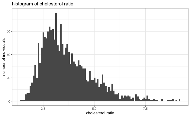
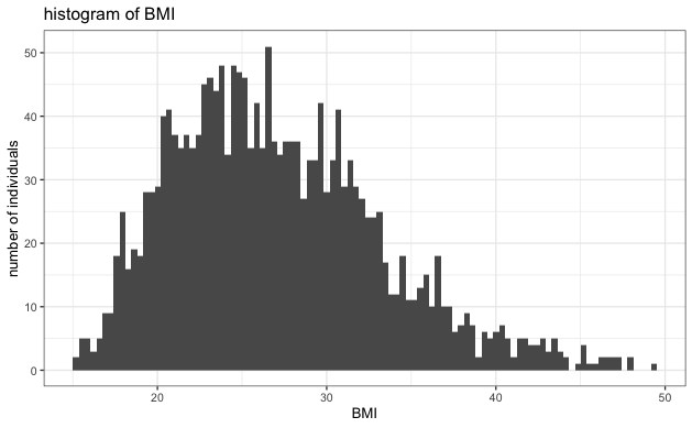
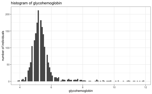
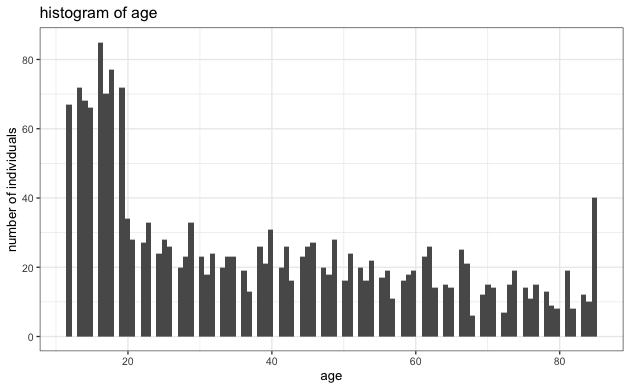
- Evaluate the normality of each variable to ensure it's not heavy-tailed. Based on the histogram below, we see no strong indication of extreme heavy-tailed distribution in any variables.
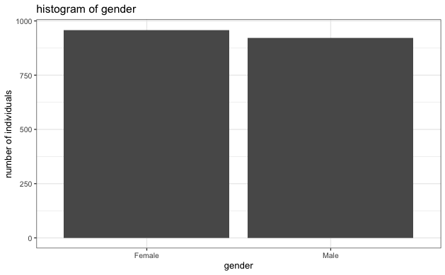
- Evaluate the number of male and female respondents to ensure there isn't a large imbalance. Based on the histogram below, the two genders are reasonably balanced.
- Check for a correlation between each independent variable and cholesterol ratio. Based on the correlation table below, each independent variable is somewhat correlated to the cholesterol ratio, with BMI being the most correlated.
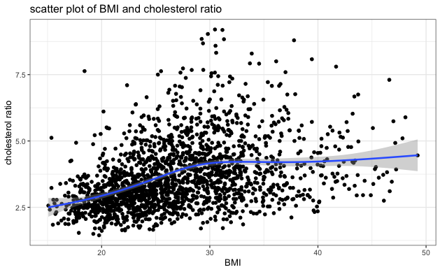
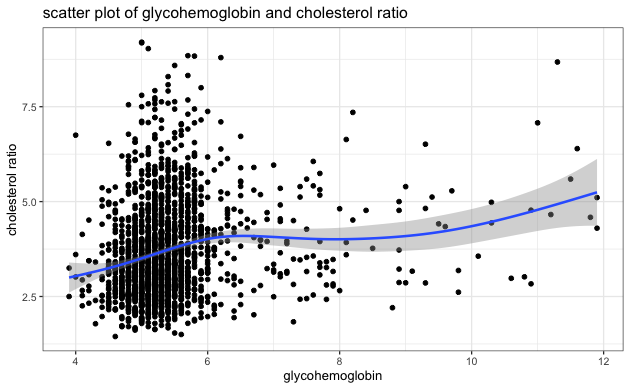
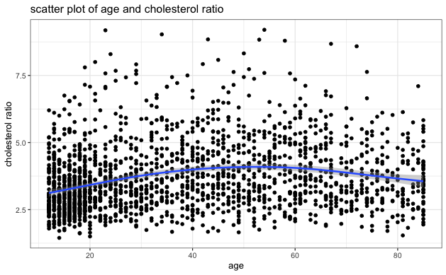
- Visually inspect the scatter plot of each independent variable and cholesterol ratio to identify any potential extreme clustering and evaluate the relationship between each independent variable and cholesterol ratio. The blue line on each plot indicates the general relationship trend between the two variables. Based on the scatter plots below, we can see no extreme clustering, and BMI has a positive relationship with cholesterol ratio, consistent with the correlation table above.
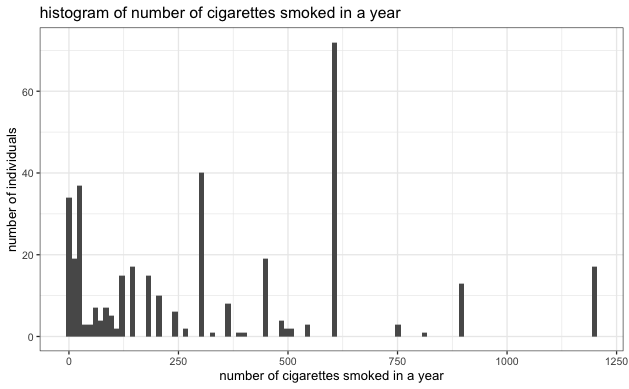
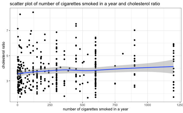
- Similar EDA steps as above were performed on the smoking dataset. There was no heavy tail distribution in the smoking dataset, but the correlation between the number of cigarettes smoked in a year and the cholesterol ratio was also relatively low, as indicated in the scatter plot below.
| Independent Variables | Correlation With Cholesterol Ratio |
|---|---|
| BMI | 0.3712956 |
| Glycohemoglobin | 0.1711966 |
| Age | 0.1791255 |
| Gender | -0.2011416 |
MODEL
With cholesterol ratio as the dependent variable and BMI as the primary independent variable, considering our large sample size and the fact that there was no strong indication of a non-linear relationship between BMI and cholesterol ratio (per scatter plot), we developed Large Sample Ordinary Least Squares (OLS) Regression models of the form:
where \(\beta_1\) represents the increase in cholesterol ratio for each unit increase in BMI, \(Z\) is a row vector for additional covariates, and \(\gamma\) is a column vector for coefficients.
We generated multiple models by adding one covariate at a time to evaluate the effects on cholesterol ratio. The model results (as generated from the confirmation set) are in the Stargazer table below. The key coefficient on BMI was highly statistically significant in all models (as indicated by the *** next to the numbers). In the default model without any covariates, each unit of increase in BMI increased the cholesterol ratio by 0.064. Each additional covariate (glycohemoglobin, age, and gender) was also highly statistically significant in all models and contributed to improving the explanatory power of the models (as evidenced by the increase in adjusted \(R^2\)). Robust standard errors were presented in parenthesis in the models to account for any possible heteroskedastic errors.
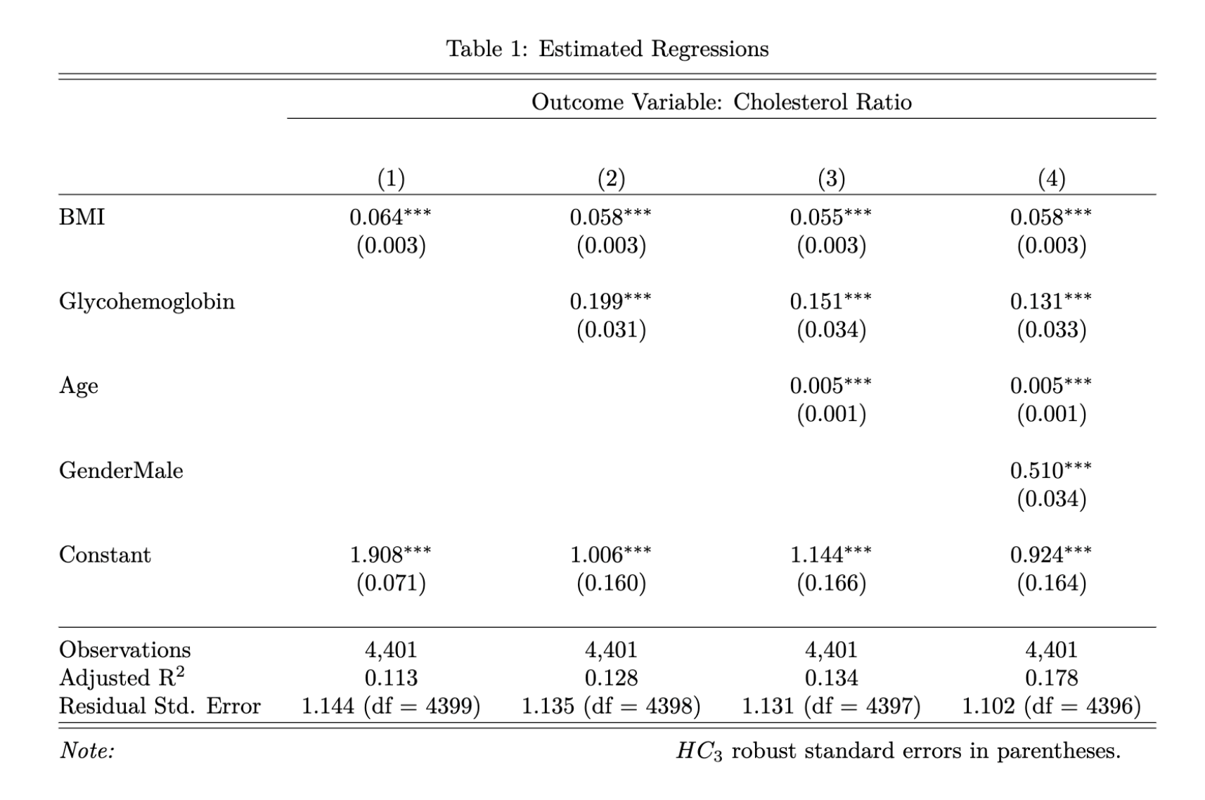
To interpret the model results, let's consider a 40-year-old female with a normal glycohemoglobin of 5.5% and a healthy BMI of 20. According to model 4, her cholesterol ratio would be 3 (20*0.058 + 5.5*0.131 + 40*0.005 + 0*0.510 + 0.924), which is highly desirable. To put this into context, a total cholesterol of 150 mg/dL with HDL of 50 mg/dL would yield a cholesterol ratio of 3. However, if her BMI were to increase to 35 (Class 1 obesity), her cholesterol ratio would increase to 3.9 (35*0.058 + 5.5*0.131 + 40*0.005 + 0*0.510 + 0.924). By age 60, assuming she had maintained the same BMI of 35 and glycohemoglobin of 5.5%, her cholesterol ratio would increase to 4 (35*0.058 + 5.5*0.131 + 60*0.005 + 0*0.510 + 0.924). A male individual of the same age with the same BMI and glycohemoglobin would have a cholesterol ratio of 4.5 (35*0.058 + 5.5*0.131 + 60*0.005 + 1*0.510 + 0.924), which would be borderline concerning. And if he is diabetic, his cholesterol ratio would be even higher.
The result emphasizes the significance of maintaining a healthy BMI to lower cholesterol ratio, especially as one age. It also suggests that those with type 2 diabetes should pay special attention to their cholesterol ratio and that males should be more mindful of their cholesterol ratio than females.
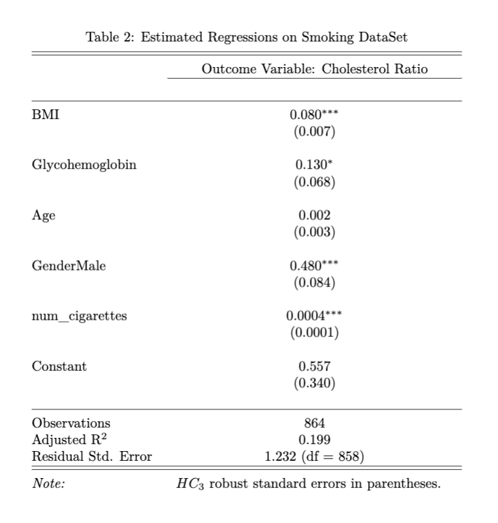
We also generated a similar regression model by including the number of cigarettes one smoked in a year as an additional covariate. The results are in the Stargazer table below. We can see that smoking, BMI, glycohemoglobin, and gender are statistically significant on cholesterol ratio. Among those who have smoked more than 100 cigarettes in their lifetime, holding all other factors constant, an additional 100 cigarettes smoked per year could lead to a 0.04 (100*0.0004) unit increase in cholesterol ratio. The inclusion of smoking habits further increased the explanatory power of the model, as evidenced by the increase in adjusted \(R^2\). However, we caution that the results from this model may not be generalizable to the population due to limitations in our sample, which excluded individuals who did not report their smoking history or who have never smoked. Further research with more representative samples is needed to draw definitive conclusions on the impact of smoking on cholesterol ratio.
LIMITATIONS
Large Sample Ordinary Least Squares Regression Model Assumptions
- Independent and identically distributed (iid) samples
- Geographic Clustering: When collecting data, individuals were sampled from counties across the United States.
- Referral: Individuals may have referred friends and relatives to complete the survey.
- When collecting data, technicians deliberately oversampled individuals of certain ages and demographics to have a more accurate representation of the United States population, which may reduce some of the iid violations
- A unique Best Linear Predictor exists
- No Extreme heavy-tailed distributions: As can be seen in the histograms, there were no extreme heavy-tailed distributions
- No perfect collinearity: There was no perfect collinearity within the independent variables, as no independent variables were automatically dropped.
- No multicollinearity: Generally, a variance inflation factor of more than 5 would indicate high multicollinearity within the independent variables. Based on the variance inflation factor table below, we can see that no independent variables exhibited evidence of multicollinearity.
Potential violations:
Justification:
| BMI | Glycohemoglobin | Age | Gender |
|---|---|---|---|
| 1.104430 | 1.217167 | 1.202331 | 1.009282 |
Omitted Variables
| Name | Description | Hypothesis | Bias | Effects |
|---|---|---|---|---|
| Familial Hypercholesterolemia | A genetic disorder | Individuals with familial hypercholesterolemia are known to have higher cholesterol ratios than those without | Positive | Driving the results away from zero and making our estimates overconfident |
| Drinking Habits | The number of alcoholic drinks an individual consumes regularly | The more alcoholic drinks an individual consumes regularly, the higher their cholesterol ratios would be | Positive | Driving the results away from zero and making our estimates overconfident |
In addition to familial hypercholesterolemia and drinking habits, we also considered the possibility of diet and physical activities as omitted variables, but as an individual's diet and physical activities directly contribute to their BMI, the effect of diet and physical activities was already reflected by BMI. Therefore, we do not believe diet and physical activities are omitted variables in our analysis.
Reverse Causality
We also acknowledge the possibility of reverse causality, where an individual's cholesterol ratio could affect their glycohemoglobin levels. Although the relationship between high cholesterol and diabetes is under debate, we recognize that the positive reverse causality bias could result in overconfident estimates. We do not believe BMI is an outcome variable of any covariates in our model.
Explanatory Power
It's important to note that our adjusted \(R^2\) was below 20%, indicating there may be other factors, such as genetics and family history, with stronger effects on cholesterol ratio. Unfortunately, our sample did not contain reliable information on these variables, which limited our ability to include them in our analysis. Future researchers may consider exploring these factors in more detail.
GITHUB
Please see my GitHub for the code and final report for the project.
MEMBER CONTRIBUTION
For the confidentiality of the team members, I will designate them as Member A, Member B, and Member C. As the sole team member without a full-time job during the project's execution, I undertook a substantial portion of the workload. Nevertheless, the project would not have been possible without every member of the team working together! Thank you all!
- Rachel: Find dataset, propose research question, data cleaning, EDA, model, report (data & methodology, results, limitations), slides (Model & Results)
- Member A: Review cleaned data & model, report (introduction & conclusion), slides (Data)
- Member B: Review cleaned data & model, report (limitation), slides (Limitation & Conclusion)
- Member C: Review cleaned data & model, slides (Introduction & Research Question)