DESCRIPTION · BACKGROUND · MOTIVATION · DATA SOURCE · DATA PROCESSING · EDA · MODEL PREPARATION · TRAINING · INFERENCE · LIMITATIONS · GITHUB
DESCRIPTION
This project utilized various machine learning algorithms (traditional, shallow neural networks, and deep neural networks) to classify bird species based on bird songs/calls. Data was sourced from the BirdCLEF 2023 kaggle competition, and all data cleaning, analysis, and model building were conducted using the Python programming language.
BACKGROUND
This was the final project for the Applied Machine Learning class in my Masters in Data Science program. The original project involved four team members including myself, for the showcase here, I have only presented the work I have done, unless noted otherwise.
The project was very open-ended, the teams are free to select any topic of interest and any dataset pertaining to that topic, with the objective to build a machine learning model.
All work was done in Google Colab (Free), with Python as the programming language. For training the deep neural networks (FFNN, CNN, and RNN), GPU is recommended to speed-up the processing time. Notable Python packages used:
- standard: numpy, pandas
- audio processing: librosa
- modeling: scikit-learn, tensorflow
- visualization: matplotlib, seaborn
MOTIVATION
During the kickoff, the team proposed a number of different ideas for the project. In addition to the bird song classifier project we ultimated landed on, the team also debated working on computer vision, regression, or NLP projects. We ultimated landed on an audio classifier project for below reasons:
- We would like to work with unstructured data.
- We all intended to take further classes on computer vision and NLP so we'd like to save computer vision and NLP projects to a later time.
- We would like to work on a project that would be better suited for deep neural networks.
Once the team agreed on pursuing an audio classifier project, we each searched for datasets containing audio data and agreed unanimously that a bird song classifier is both interesting and challenging enough for our project.
While no team member came from a biosience background, it was interesting to learn that scientists often carry out observer-based surveys to track changes in habitat biodiversity. These surveys tend to be costly and logistics challenging, while a machine learning-based approach that can identify bird species using audio recordings would allow scientists to explore the relationship between restoration interventions and biodiversity on a larger scale, with greater precision, and at a lower cost.
DATA SOURCE
We obtained our data from the BirdCLEF 2023 kaggle competition hosted by the Cornell Lab of Ornithology. For the competition, the training dataset contained short recordings of individual bird calls for 264 different bird species across the globe. The audio recordings were sourced from xenocanto.org and all audio files were downsampled to 32 kHz where applicable and stored in the ogg format.
In addition to audio recordings of the bird calls, the training data also contained additional metadata such as secondary bird species, call type, location, auality rating, and taxonomy. The test labels were hidden for the submission purpose. Below is the first 5 rows of the training data as provided by the competition.
| primary_label | secondary_labels | type | latitude | longitude | scientific_name | common_name | author | license | rating | url | filename |
|---|---|---|---|---|---|---|---|---|---|---|---|
| abethr1 | [] | ['song'] | 4.3906 | 38.2788 | Turdus tephronotus | African Bare-eyed Thrush | Rolf A. de By | Creative Commons Attribution-NonCommercial-ShareAlike 3.0 | 4.0 | https://www.xeno-canto.org/128013 | abethr1/XC128013.ogg |
| abethr1 | [] | ['call'] | -2.9524 | 38.2921 | Turdus tephronotus | African Bare-eyed Thrush | James Bradley | Creative Commons Attribution-NonCommercial-ShareAlike 4.0 | 3.5 | https://www.xeno-canto.org/363501 | abethr1/XC363501.ogg |
| abethr1 | [] | ['song'] | -2.9524 | 38.2921 | Turdus tephronotus | African Bare-eyed Thrush | James Bradley | Creative Commons Attribution-NonCommercial-ShareAlike 4.0 | 3.5 | https://www.xeno-canto.org/363502 | abethr1/XC363502.ogg |
| abethr1 | [] | ['song'] | -2.9524 | 38.2921 | Turdus tephronotus | African Bare-eyed Thrush | James Bradley | Creative Commons Attribution-NonCommercial-ShareAlike 4.0 | 5.0 | https://www.xeno-canto.org/363503 | abethr1/XC363503.ogg |
| abethr1 | [] | ['call', 'song'] | -2.9524 | 38.2921 | Turdus tephronotus | African Bare-eyed Thrush | James Bradley | Creative Commons Attribution-NonCommercial-ShareAlike 4.0 | 4.5 | https://www.xeno-canto.org/363504 | abethr1/XC363504.ogg |
Notably, at the time of this project, the BirdCLEF 2023 competition had already ended, so the goal of the project was not to create a model for the competition submission, but rather to use the dataset to create a bird species classifier using machine learning techniques.
Since the audio data for all 264 species are too large to fit into Google Colab free version, we reduced the scope of the task and only selected 3 species from 3 different families to build a bird song classifier for the 3 selected species. As the test data provided by the competition contained unknown labels, we did not use the test data provided by the competition for our project. Instead, we split the training data to training, validation, and test sets for building our machine learning models.
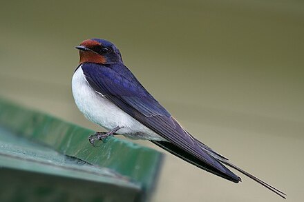
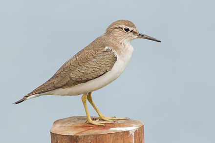
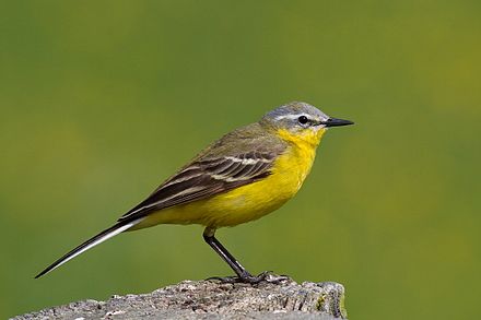
The 3 species selected for the project are as follows:
DATA PROCESSING
A. Data Preprocessing
Summarized below are the top level data preprocessing steps I performed, the Google Colab notebook shown in the video is the a.preprocessing.ipynb file in the 1.preprocessing folder of the GitHub repo.
- Include only the species selected.
- Remove duplicate.
- Train/Test split.
As noted in the previous section, only 3 species (barswa, comsan, and eaywag1) were selected for this project.
Instances with the same 'duration', 'type', 'location', 'primary_label', and 'author' appear to be duplicates and were removed from the dataset.
To prevent data leakage, the data was split to train and test dataset at 70/30 split.
Train
70%
Test
30%
B. Data Cleaning
After the top level preprocessing steps, the data was cleaned as summarized below. The Google Colab notebook shown in the videos is the b.data_cleaning.ipynb file in the 1.preprocessing folder of the GitHub repo.
- Inspect each column for NaN values.
- Inspect each column for outliers or things that would require special attention.
- Drop unused columns.
- Clean up the 'type' column.
- Extract country and continent from latitude and longitude.
Only latitude and longitude columns contained NaN values, but only 17 out of the more than 1000 training examples had NaN latitude and longitude so I just left them as is.
There wasn't outliers that really stood out in this step, but instead, I noted down some columns that should be removed and some columns that could be cleaned up a bit which I performed below.
'secondary_labels', 'scientific_name', 'common_name', 'author', 'license', and 'url' columns are not useful for our analysis so they were dropped from our data.
Some 'type' contained the bird gender and lifestage which were not related to call or song types so I summarized all types to either 'call', 'song', 'blank', or 'both'.
Part 1 (Steps 1-4)
Part 2 (Step 5)
C. Data Extraction
One thing I discovered while working on the project was that loading the audio clips using librosa.load() is time consuming. librosa.load() takes in audio files as parameter and returns the audio object in a NumPy array. The same NumPy array object can be passed as parameters to other librosa functions to extract audio features. To save downstream processing time, I used librosa.load() to load the audio files and saved the returned NumPy array object to disk, which enabled me to use the NumPy array object directly when extracting audio features. The Google Colab notebook shown in the videos is the c.data_extraction.ipynb file in the 1.preprocessing folder of the GitHub repo.
EDA
To get a better understanding of what audio features would be appropriate for this project, what EDA could be performed on the features, and what machine learning algorithms are most suited for audio classification tasks, I looked at the notebooks from prior year BirdCLEF competitions and read a number of articles/papers that used audio features to build machine learning model. Listed below are some notable resources that was considered when performing feature extraction, EDA, and model building for this project.
- BirdCLEF 2021 2nd place
- BirdCLEF 2022 1st place
- BirdCLEF 2023 1st place
- Comparative Audio Analysis With Wavenet, MFCCs, UMAP, t-SNE and PCA
- CNNs for Audio Classification
- Environment Sound Classification Using a Two-Stream CNN Based on Decision-Level Fusion
- Data Augmentation Techniques for Audio Data in Python
A. General EDA
To build more generalizable models, EDAs are performed on training set only, so as to not gaining any information from the test set.
Summarized below are some general EDA performed on the training set. The Google Colab notebook shown in the video is the a.EDA.ipynb file in the 2.EDA folder of the GitHub repo.
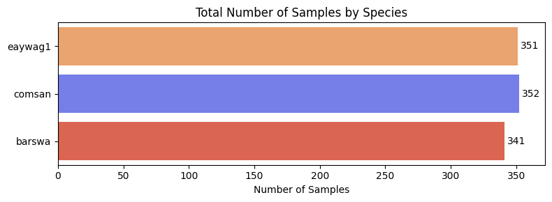
- Check for class imbalance by number of samples.
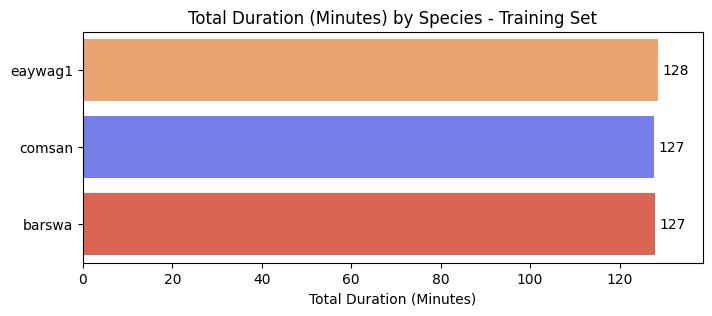
- Check for class imbalance by total duration.
- Check for total duration by call types.
- Check for total duration by quality rating.
- Check for geolocation distribution by species.
The three species are relatively balanced by number of samples, with barswa having slightly fewer number of samples than the other two, but the difference is not alarming.
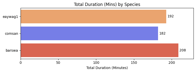
In general, we expect features to be of the same shape when passed into machine learning models as inputs. In the case of audio inputs, each audio clip should be of the same duration. Since audio clips in our dataset are of different duration, we will need to split the audio clips to a set duration before passing into the models. Therefore, I also checked for class imbalance by total duration.
At first glance, it may seem the three classes have similar total duration, however, if each audio clip is split to 5 seconds inputs without overlapping, a 10 minutes difference would result in a difference of 120 input samples. This difference would be even larger if the audio clips are split to 3 seconds clips, or if the audio clips are split with overlapping. This imbalance in total duration could result in the model favoring the species with longer duration during training. To overcome this imbalance, we can either drop some of the oversampled class (barswa), or we can stretch the audios of the undersampled classes (comsan and eaywag1) to make the three classes having similar total duration.
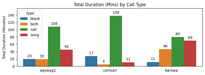
The call types were cleaned up as part of the data preprocessing steps mentioned above. While barswa made both 'call' and 'song' types almost equally, eaywag1 made more 'call' type than 'song', and comsan made almost exclusively only 'call' type. This might be useful information if we want to use call types as one of the input features.
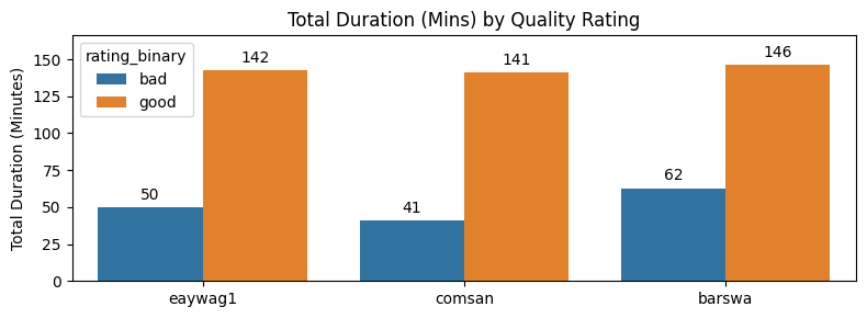
In the original dataset, the quality rating attribute is on a scale of 0.0-5.0, presumably with 0.0 being the worst quality and 5.0 being the best quality. To better visualize the quality rating, I turned the attribute to binary, with audios of ratings above 3.0 being 'good'. All three classes had similar total durations of 'good' quality recordings, while barswa had more 'bad' quality recordings than the other two. Downsampling the 'bad' quality barswa recordings could be another way to overcome the class imbalance by total duration issue mentioned above.
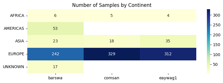
As part of the preprocessing, I extracted the continents of each audio sample based on the latitude and longitude. Majority of the audio clips were recorded in Europe with some in Asia and Africa. Interestingly, none of the comsan and eaywag1 audios were recorded in Americas, which might be a valuable distinguishing feature between barswa and the other two species.
B. Audio Features
Once the audio NumPy array objects had been extracted from the raw audio files using librosa.load(), they were passed as parameters to various librosa feature extraction functions to extract the relevant audio features. Below summarized are some of the key audio features commonly used for audio classification tasks, in particular, MFCC and melspectrograms appear to be the most useful based on existing research.
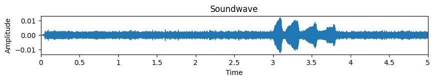
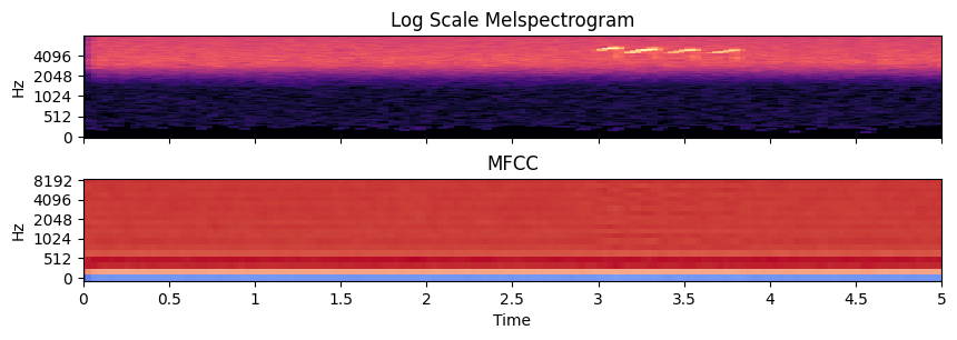
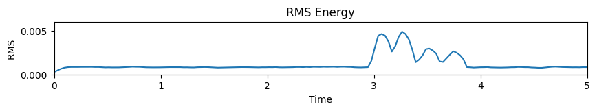
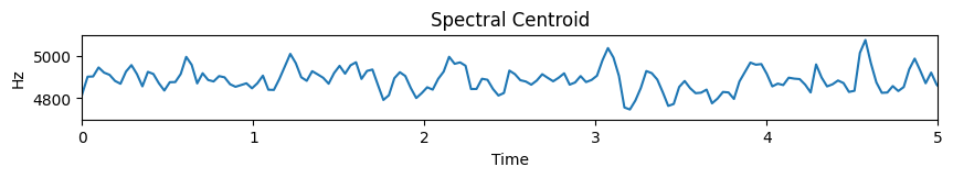
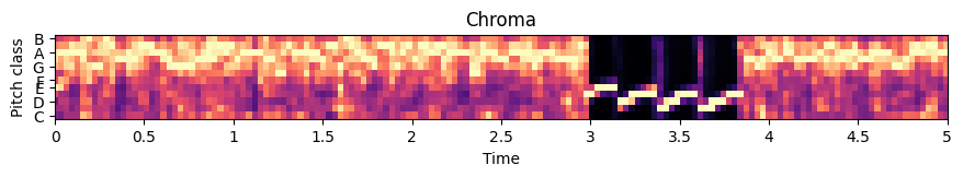
Here is a visual representation of the different features derived from the 5 second audio clip below. The code used to generate this visualization can be found in the b.audio_features.ipynb file in the 2.EDA folder of the GitHub repo.
- Soundwave.
- Melspectrogram & Mel-Frequency Cepstral Coefficients (MFCC): visualization of the power distribution of audio frequencies, transformed into the mel scale to better represent human perception of sound.
- RMS energy: a measure of the signal's magnitude or "loudness" over time
- Spectral Centroid: a feature that represents the "center of mass" of the spectrum, in another word, the ‘brightness’ of the sound over time
- Chroma: a feature that summarizes the 12 different pitch classes
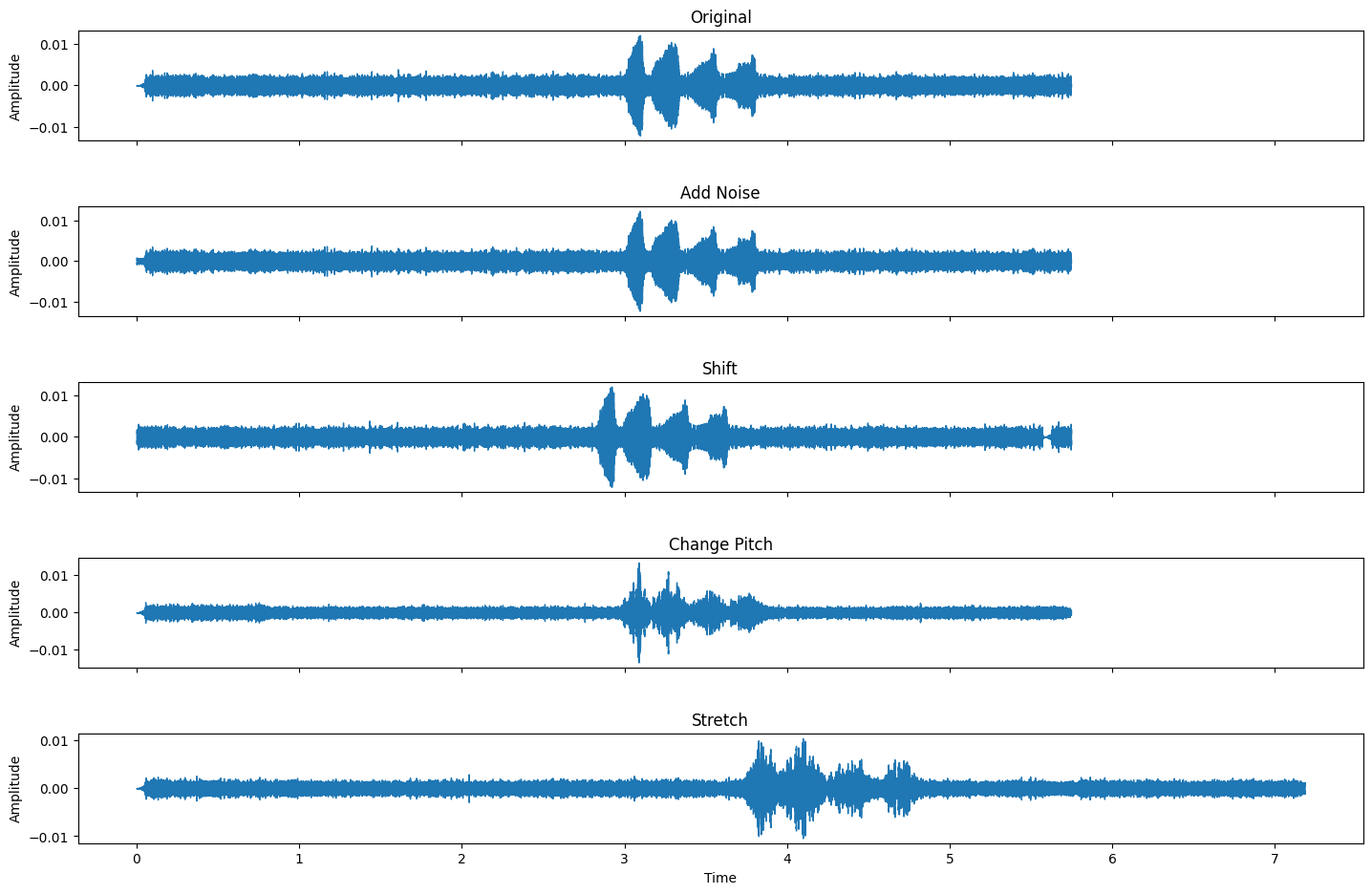
C. Audio Augmentation
Augmentation is an important consideration when working with audio data. Some common augmentation techniques are:
- Adding gaussian noise to the audio.
- Shifting the entire audio along the time axis.
- Changing the pitch of the audio.
- Stretching the entire audio along the time axis.
Below is a visual representation of how the origianl 5 second audio soundwave changes with each augmentation technique. The code used to generate this visualization can be found in the c.augmentation.ipynb file in the 2.EDA folder of the GitHub repo.
MODEL PREPARATION
A. Train/Validation Split
Since the test dataset is reserved for final inference purpose, I further split the training dataset to train and validation sets for hyperparameter tuning during training. The code used to split the training dataset can be found in the a.train_val_split.ipynb file in the 3.model_prep folder of the GitHub repo.
Train
70%
Test
30%
Train
70%
Val
30%
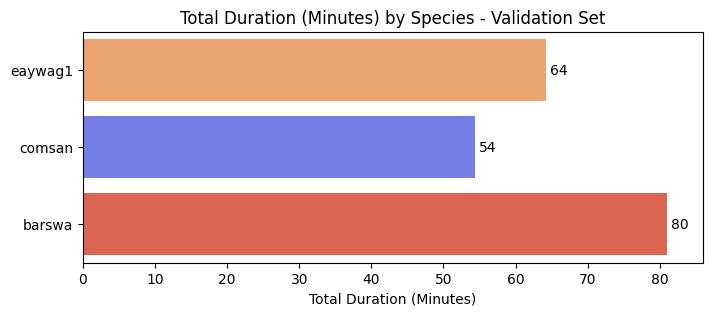
To overcome the class imbalance in total duration, I downsampled the oversampled species in training set and put the rest in validation set. By doing this, the training set is now balanced, which would allow the models to learn features from the three classes equally well during training.
The total duration in the validation set is imbalanced after splitting to train/val sets, as it should be representative of the potential imbalance in the test set.
B. Create Class Methods
Even though only 3 species were selected for the project, the audio features for the training and validation set are still too large to fit into memory of Google Colab (the free version only provides 12.7GB RAM). I therefore created two class methods which allowed me to manage the memory usage more efficiently.
The Framed class is used to frame the audios (split audios of varying length to set lengths clips with or without augmentation, and with or without overlapping). The Extraction class is used to extract the audio features and labels from each of the framed clips (with or without normalization and/or average pooling) in a shape that's ready to be passed into the models. The code used to create and test the class methods can be found in the b.class_methods.ipynb file in the 3.model_prep folder of the GitHub repo.
Part 1 (Train/Val split & class methods)
C. Extract Framed Audios
Since I intend to experiment various machine learning algorithms, it would be inefficient to frame the audios and extract the features everytime in each model notebook. Therefore, I used the Framed class (discussed above) to extract the framed audios with below specifications and saved the updated dataframe (including the 'framed' column) to disk for future use.
- 5.0 seconds frame with 2.5 seconds overlap - with and without augmentation
- 8.0 seconds frame with 4.0 seconds overlap - with and without augmentation
Usually, pandas dataframes can be saved to disk in csv format to be reloaded as dataframes when needed, however, since the framed audios are framed using the tf.signal.frame method which returns the framed audios as an array of Tensor objects, saving arrays of Tensor objects to csv format would render the objects unusuable (or at least very difficult to parse). So, in order to save the updated dataframe in a reloadable format, the dataframes were saved to disk using the pickle library in pkl format. The code used to extract the framed audios and save the updated dataframes can be found in the c.extract_framed_audios folder in the 3.model_prep folder of the GitHub repo.
D. Extract Features & Labels
Once the framed audios have been extracted, I then used the Extraction class (discussed above) to extract the various features with below specifications (all numeric features were normalized), and then saved the extracted features to disk (using pickle) for future use. The numbers in parenthesis indicate the number of each feature extracted from each audio. The code used to extract and save the features can be found in the d.extract_features_labels folder in the 3.model_prep folder of the GitHub repo.
- MFCC(20) with and without average pooling
- Chroma(12) with and without average pooling
- RMS(1) with and without average pooling
- Spectral Centroid(1) with and without average pooling
- Melspectrogram(20) with and without average pooling
- Continent
- Type
- Rating
Part 2 (Extract framed audio & features)
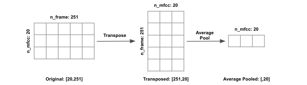
To better understand the dimension of the audio features, let's assume we have one audio sample of 8 seconds in duration, sampled at 16000 sample_rate. The audio input signal would then have shape [n,] where n = (duration_in_seconds * sample_rate) = (8 * 16000) = 128000. The number of frames (n_frame) can then be calculated as (n / hop_length + 1) = (128000 / 512 + 1) = 251, where hop_length is default to window_length // 4 = 2048 // 4 = 512, where window_length is default to 2048 in librosa. If we then extracted 20 MFCCs at each time step, the resulting MFCC feature dimension would be [n_frame, n_mfcc] = [251, 20]. It's worth noting that the features returned from librosa feature extraction functions takes on dimension of [n_feature, n_frame] by default, I transposed the features to take on dimension of [n_frame, n_feature] instead so average pools and convolutions are applied along the time axis.
When average pooling is applied, each audio feature of shape [n_frame, n_feature] are average pooled along the time axis, resulting in audio feature of shape [,n_feature]. In our example, the 8 seconds audio sample with 20 MFCCs would produce an average pooled feature of shape [,20]. We can therefore view average pooling as a dimensionality reduction technique, where a 2D feature of shape [251, 20] is reduce to 1D of shape [,20] by taking the average of the 251 frames for each MFCC. This process can be visualized as below.
When average pooling is not applied, each audio feature of shape [n_frame, n_feature] keeps its original dimension. If we have 100 8-seconds samples, each with 20 MFCCs, our inputs with average pooling would then have dimension [n_samples, n_features] = [100, 20], our inputs without average pooling would then have dimension [n_samples, n_frame, n_features] = [100, 251, 20]. If we were to extract and concatenate more than one feature, let's say 20 MFCCs and 12 Chroma, our 100 sample inputs would then have dimension [100, 32] with average pooling, or [100, 251, 32] without average pooling, where 32 = 20 MFCCs + 12 Chroma.
TRAINING
Baseline · Random Forest · XGBoost · SVM · Logistic Regression · FFNN · 1D CNN · 2D CNN · LSTM RNN · GRU RNN · Transformer · Transfer Learning
A1. Baseline
Each species represent 1/3 of the total duration in the training set, if one were to randomly guess the species, we would expect a 33% accuracy. This will serve as our baseline.
All notebooks for the models can be found in the 4.training folder in the GitHub repo.
B1. Ensemble - Random Forest
Ensemble is a machine learning technique that combined multiple models to one model. Random Forest, rooted from decision tree, is one of the ensemble techniques, where multiple decision trees are used to find the most optimal predictive feature at each 'branch'. I used the RandomForestClassifier from sklearn to implement the random forest models.
As mentioned earlier, many different audio features (such as MFCC, RMS, etc) could be extracted and used as features in machine learning models, so I implemented random forest models with 16 different combinations of various features to find the features with the strongest predictive power. I also experimented with different framed audio duration (3 seconds with 1 second overlap, 5 seconds with 2.5 seconds overlap, and 8 seconds with 4 seconds overlap) in case the audio frame duration made a difference in the models.
Summarized below are the feature combinations from the models with the highest validation accuracy for each framed audio duration, with no augmentation. All models were generated with 50 estimators, with entropy as the criterion, and with combinations of normalized and average pooled (along time axis) 20 MFCC, 20 melspectrogram, 12 chroma, 1 RMS, 1 spectral Centroid, and/or 5 one-hot encoded continents.
| Framed Duration (secs) | Overlap Duration (secs) | Features | Training Accuracy | Validation Accuracy |
|---|---|---|---|---|
| 3.0 | 1.0 | MFCC(20) + Spectral_Centoid(1) + Continents(5) | 100% | 69% |
| 3.0 | 1.0 | MFCC(20) + RMS(1) + Continents(5) | 100% | 69% |
| 5.0 | 2.5 | MFCC(20) + Continents(5) | 100% | 69% |
| 5.0 | 2.5 | MFCC(20) + Chroma(12) + Continents(5) | 100% | 70% |
| 8.0 | 4.0 | MFCC(20) + Spectral_Centoid(1) + Continents(5) | 100% | 71% |
| 8.0 | 4.0 | MFCC(20) + RMS(1) + Continents(5) | 100% | 73% |
From this summary, we can see MFCC is predominently a better predictor than melspectrogram, and MFCC + continents are the strongest predictor among all combinations. The predictive power of RMS, chroma, and spectral centroid is not conclusive from this exercise alone, and even though framed audios with 8 seconds in length had the highest validation accuracy, the different to that of 5 seconds is not glaring so I would not conclude framed audios with 8 seconds in length are better than those with 5 seconds in length (at least not just yet). Notabily, framing audios to 3 seconds created more training samples, but did not improve the results. Going forward, I will only work with framing duration of 5 seconds or 8 seconds.
I also tried applying random augmentation to the training samples for the 5 seconds and 8 seconds framed samples, but it did not improve the model performance. This is not to say augmentation is not useful, but rather the augmentation technique may need to be revisited. I also tried increasing the number of melspectrogram to 128 (instead of 20) which did not make a difference in model performance.
The best performing model had 73% validation accuracy, which is much higher than our baseline of 33% (random guess), the algorithm is performing better than I expected but consistent with the general characteristics of random forest, all models are severely overfitted to the training data. For hypertuning the models, I changed the number of estimators to 40 and 80. Neither change made notable difference in the model performance. I did not hypertune the criterion as my research suggested entropy is generally the better criterion to use.
B2. Ensemble - XGBoost
XGBoost is another ensemble machine learning technique that utilizes the gradient boosting framework to provide parallel tree boosting in decision tree algorithms. I used the Framed and Extraction classes for framing the audios and extracting the features in the random forest notebooks, but starting from XGBoost, I will be directly using the features saved in .pkl format to improve efficiency.
Similar to the random forest models, I experimented with different combinations of features from 5 seconds framed audios and 8 seconds framed audios, with and without augmentation. Summarized below are the feature combinations from the models with the highest validation accuracy for each framed audio duration. All models were generated with 100 estimators, with dart as the booster.
| Framed Duration (secs) | Overlap Duration (secs) | Features | Augment | Training Accuracy | Validation Accuracy |
|---|---|---|---|---|---|
| 5.0 | 2.5 | MFCC(20) + Chroma(12) + Continents(5) | No | 100% | 70% |
| 5.0 | 2.5 | MFCC(20) + Chroma(12) + Continents(5) | Yes | 100% | 69% |
| 8.0 | 4.0 | MFCC(20) + RMS(1) + Continents(5) | No | 100% | 72% |
| 8.0 | 4.0 | MFCC(20) + RMS(1) + Continents(5) | Yes | 100% | 72% |
Similar to the findings from the random forest models, MFCC is predominently a better predictor than melspectrogram, and MFCC + chroma or MFCC + RMS together with continents are consistently the better predictor than any other feature combinations. The 8 seconds framed audios again had higher validation accuracy than those with 5 seconds, and the random augmentation applied to the audios did not play a role in improving the models. The models had similar performance as random forest and are still severely overfitted to the training data.
For hypertuning the models, I used GridSearchCV from sklearn. The GridSearch was ran on the model with the same specifications as the highlighted model above. I also ran another model with the same specifications but replaced RMS with chroma. The GridSearch identified the best max depth at 6 with 200 estimators. However, the validation accuracy with this optimal hyperparameter setting did not improve over the original model, this is expected as the model is overfitted to the training data and already learned 100% of the features in the training data in the original model (with fewer estimators). To improve the model, more training data is likely needed.
C1. Support Vector Machine (SVM)
Another tranditional machine learning algorithm commonly used for classification tasks is support vector machine (SVM), which is an algorithm used to identify a hyperplane that segregates/classifies the data points in an N-dimensional space. I used SVC from sklearn to implement the SVM models.
I again experimented with different combinations of features from 5 seconds framed audios and 8 seconds framed audios, with and without augmentation. Summarized below are the feature combinations from the models with the highest validation accuracy for each framed audio duration. All models were generated with C=4 (regularization parameter), with rbf as the kernel.
| Framed Duration (secs) | Overlap Duration (secs) | Features | Augment | Training Accuracy | Validation Accuracy |
|---|---|---|---|---|---|
| 5.0 | 2.5 | MFCC(20) + Chroma(12) + Continents(5) | No | 90% | 72% |
| 5.0 | 2.5 | MFCC(20) + Chroma(12) + Continents(5) | Yes | 87% | 69% |
| 8.0 | 4.0 | All Features | No | 92% | 74% |
| 8.0 | 4.0 | MFCC(20) + Chroma(12) + Continents(5) | Yes | 87% | 72% |
The results are still consistent with the findings from the previous two models so I will omit detailed discussion here. Notabily SVM was much faster to run than XGBoost and the training results are less overfitted with comparable validation accuracy. For hypertuning the models, I again used GridSearchCV from sklearn. The hypertuning did not improve the performance of the models.
D1. Logistic Regression
Logistic regression is perhaps the most basic machine learning algorithm for classification tasks. Similar to the earlier models, I experimented with different combinations of features from 5 seconds framed audios and 8 seconds framed audios, with and without augmentation. Summarized below are the feature combinations from the models with the highest validation accuracy for each framed audio duration. All models used Adam optimizer, 0.005 learning rate, batch size of 32, and ran for 100 epochs.
| Framed Duration (secs) | Overlap Duration (secs) | Features | Augment | Training Accuracy | Validation Accuracy |
|---|---|---|---|---|---|
| 5.0 | 2.5 | MFCC(20) + Spectral Centroid(1) + Continents(5) | No | 70% | 65% |
| 5.0 | 2.5 | MFCC(20) + RMS(1) + Continents(5) | Yes | 68% | 60% |
| 8.0 | 4.0 | MFCC(20) + Spectral Centroid(1) + Continents(5) | No | 72% | 65% |
| 8.0 | 4.0 | MFCC(20) + RMS(1) + Continents(5) | Yes | 71% | 65% |
As expected, the logistic regression models performed poorly (still better than baseline but worse than any of the previous traditional machine learning algorithms), they are less overfitted (which is good), but the validation accuracy are consistently lower than prior models. Logistic regression is generally better suited for simpler classification tasks, where the data is linearly separable, which is rarely the case for most real life datasets. But nevertheless, I wanted to give it a try so I can compare the performance between shallow neural network (logistic regression) and deep neural networks (FFNN, CNN, etc).
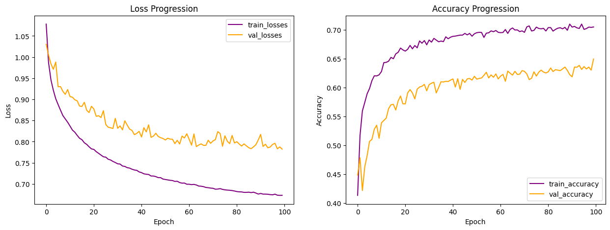
To visualize the learning progress for the best performing logistic regression model (highlighted above), I plotted the below loss and accuracy progression curves for training and validation over the 100 epochs. We can see the model is making steady learning progress one epoch after another. The validation curve is pretty far apart from the training curve, indicating signs of overfitting. I also observed the zig zag pattern in the learning curves, more prominently in the validation curves, indicating the performance is unsteady, a sign that the model is struggling with the validation data one epoch after another. I should expect the two learning curves (train and validation) be closer together, with less zig zag, with a more complex architecture.
I did not bother hypertuning the models as I know logistic regression is not the best suited algorithm for the data.
E1. Feed Forward Neural Network (FFNN)
The first deep neural network I tried is Feed Forward Neural Network (FFNN), it is essentially a logistic regression model but with hidden layers added. The hidden layers (actived with some non-linear activation function) allow the model to find non-linear relationships between the features and the labels.
Based on observations from the models above, it appears framed audios with 8 seconds in duration without augmentation have consistently outperformed others, so I will be using 8 seconds framed audios going forward. This is not to say other durations are inferior, it's just for this dataset (and with the way I processed the data), framing audios to 8 seconds seems to work better. Similarly, models with MFCC as the primary audio feature have consistently outperformed those with melspectrogram, so I will also be using only MFCC as the primary audio feature going forward. Again, many other audio models have found success in using melspectrogram and I have no doubt it is equally good or even better than MFCC, it's just I've had better performance with MFCC for this project so far.
Summarized below are the results with different feature combinations. All models used Adam optimizer, 0.0001 learning rate, batch size of 32, ran for 100 epochs, with 3 hidden layers, each of 128, 64, and 32 nodes respectively and activated with the ReLU activation function.
| Features | Training Accuracy | Validation Accuracy |
|---|---|---|
| MFCC(20) + RMS(1) + Spectral Centroid(1) | 81% | 66% |
| MFCC(20) + RMS(1) + Continents(5) | 79% | 69% |
| MFCC(20) + Spectral Centroid(1) + Continents(5) | 81% | 71% |
| MFCC(20) + Chroma(12) + Continents(5) | 84% | 75% |
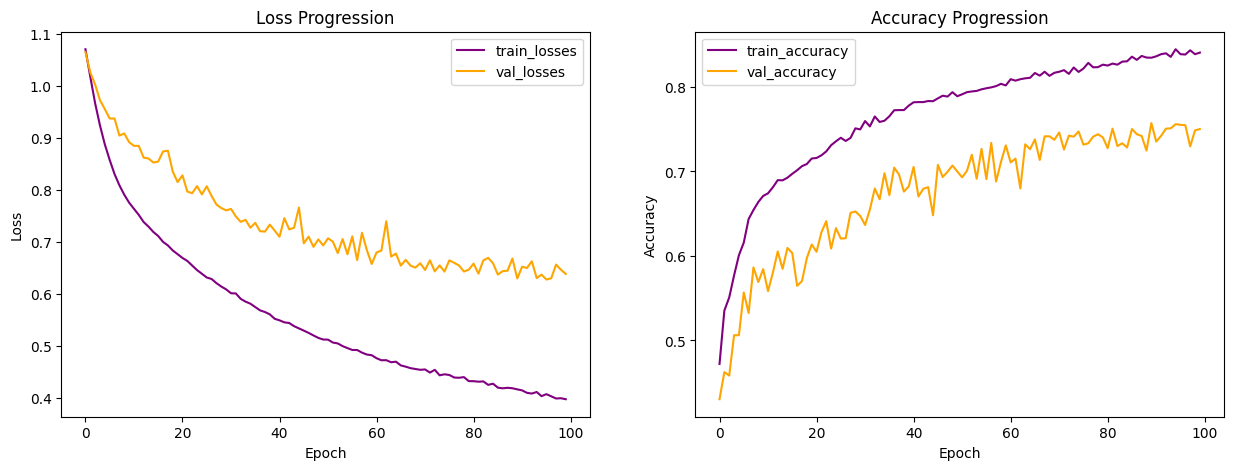
Compared to logistic regression and all prior models, FFNN had the highest validation accuracy and was the least overfitted. Below is the learning curves from the best performing model (highlighted above). Compared to the learning curves from logistic regression above, we still observe the zig zag in the validation curves, suggesting the model is still struggling with the validation data from one epoch to another.
To better understand how each hyperparameter changes the model performance, I did an ablation study on the best performing model (highlighted above) by changing the learning rate, batch size, number of epochs, the number of hidden layers, and the number of nodes in each hidden layer. Summarized below is the results from the ablation study, the study is not exhaustive but based on the study, the default hyperparameter settings (Adam optimizer, 0.0001 learning rate, batch size of 32, ran for 100 epochs, with 3 hidden layers, each of 128, 64, and 32 nodes) performed the best with this dataset. The validation accuracy changed slightly from the original model (highlighted above) due to randomness in initial weight initialization and shuffling.
| Hidden Layer | Num Epochs | Batch Size | Learning Rate | Training Accuracy | Validation Accuracy |
|---|---|---|---|---|---|
| [128,64,32] | 100 | 32 | 0.0001 | 0.84 | 0.77 |
| [32] | 100 | 32 | 0.0001 | 0.67 | 0.56 |
| [64,32] | 100 | 32 | 0.0001 | 0.77 | 0.66 |
| [256,128,64] | 100 | 32 | 0.0001 | 0.91 | 0.74 |
| [128,64,32] | 200 | 32 | 0.0001 | 0.90 | 0.73 |
| [128,64,32] | 100 | 8 | 0.0001 | 0.88 | 0.71 |
| [128,64,32] | 100 | 64 | 0.0001 | 0.82 | 0.71 |
| [128,64,32] | 100 | 32 | 0.01 | 0.88 | 0.70 |
| [128,64,32] | 100 | 32 | 0.0005 | 0.92 | 0.68 |
F1. 1D Convolutional Neural Networks (1D CNN)
Similar to FFNN models implemented above, I implemented the 1D CNN models with tensorflow functional API architecture, with 8 seconds framed audios, MFCC as the main audio feature, and without augmentation.
Different from FFNN (and any other models implemented above), the audio features are no longer average pooled, but instead kept in the original 2D dimension, to be convoluted along the time axis. To the right is an animated illustration of 1D convolute along the time axis for an 8-second audio sample (at 16000 sample rate) with 20 MFCC and 12 chroma features, the features are concetenated and the yellow box represents one filter.
Also different from previous models, instead of one hot encoding the continents, I decided to create embedding representations of the continents. Embeddings are used for natural language processing tasks as learned representations of words or tokens. Since continents are words, I thought why not give embeddings a try.
I used tensorflow keras Embedding() layer to create embeddings with output dimension 2 for the 6 tokens, each token represents one continent (there are 5 continents in our training data, including one 'unknown' continent), plus an additional token reserved for out-of-dictionary word. To make the embedding dimensions match the audio features dimensions, I tiled the embeddings along the time axis to change embeddings of shape [,embedding_dim] = [,2] to shape [n_frame,embedding_dim] = [251,2], effectively the embeddings for each continent for the respective audio sample is repeated along the time axis. Once the embeddings were tiled to the same shape as the audio features, the audio features and embeddings were concatenated, resulting in input features of shape [251, 34] in the example of 20 MFCC + 12 Chroma + 2 Embeddings.
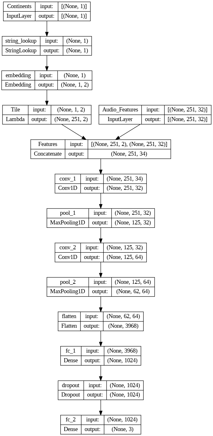
All models were ran with the same architecture: two 1D conv layers (each with kernel_size=5, strides=1, activated with the ReLU activation function, and L2 regularization=0.02, with the first layer having 32 filters and the second layer having 64 filters), each followed by a max pooling layer (each with pool_size=2), followed by a flattening layer and then a fully connected layer (with units=1024), before being passed to a 50% dropout layer, which finally leads to the output layer. In addition, I also utilized the 'rating' feature to create sample weights to give audio samples with worse ratings less weights during training. L2 regularization and dropout were employed to reduce overfitting, and callback technique was used to call the model back to the epoch with the highest weighted validation accuracy. All models were trained with the Adam optimizer, 0.001 learning rate, and batch size of 32. To the left is a visualization of the model architecture (with 20 MFCC and 12 Chroma + continents embeddings as features).
Summarized below are the results with different feature combinations, utilizing the same architecture and hyper-parameters mentioned above. Compared to all prior models, there is a clear jump in performance, from 75% highest validation accuracy (FFNN) to 91% highest validation accuracy, and the models are noticeabily less overfitted than all prior models.
| Features | Training Accuracy | Validation Accuracy |
|---|---|---|
| MFCC(20) + Chroma(12) + Continents(2) | 98% | 87% |
| MFCC(20) + Chroma(12) + RMS(1) + Spectral Centroid(1) + Continents(2) | 97% | 87% |
| MFCC(20) + Spectral Centroid(1) + Continents(2) | 98% | 90% |
| MFCC(20) + RMS(1) + Continents(2) | 98% | 91% |
| MFCC(20) + RMS(1) + Spectral Centroid(1) + Continents(2) | 97% | 91% |
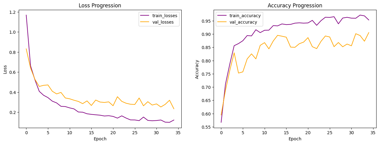
Below is the learning curves from the best performing model (highlighted above). It's worth noting that the learning curves are not exactly apple-to-apple comparison to all prior models, since I utilized callback technique when training the 1D CNN models, so the progression is only up until the best epoch (epoch 35) here.
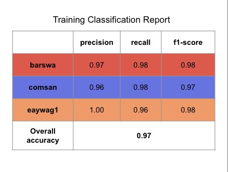
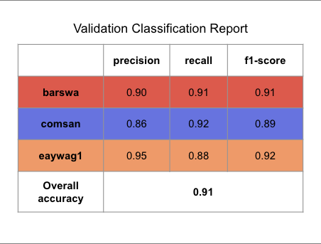
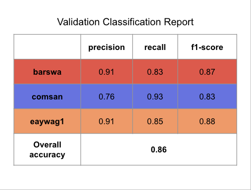
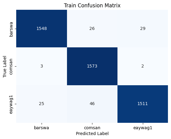
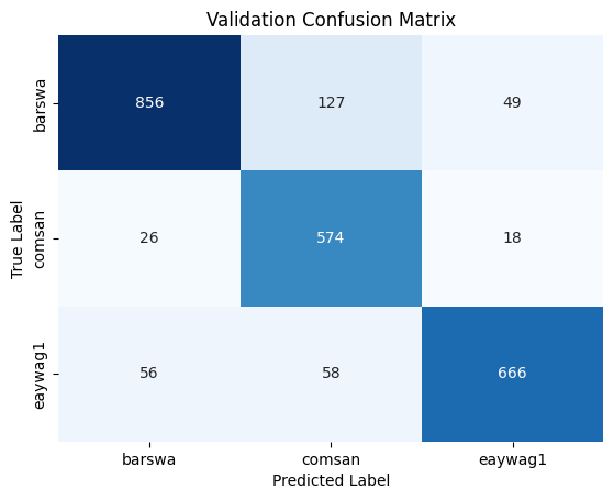
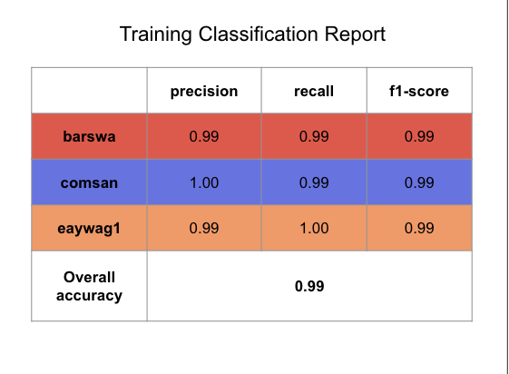
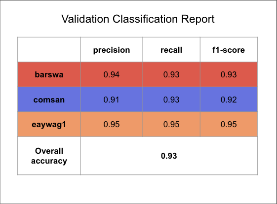
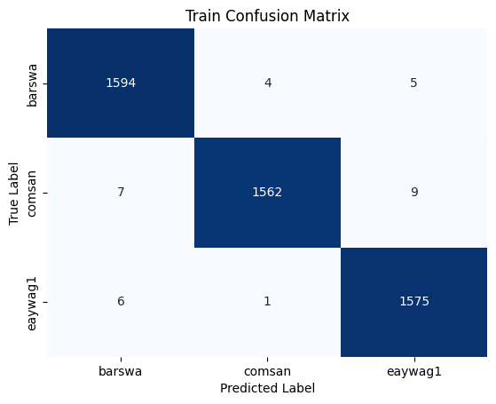
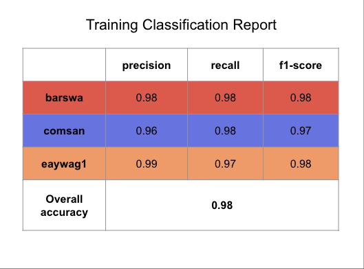
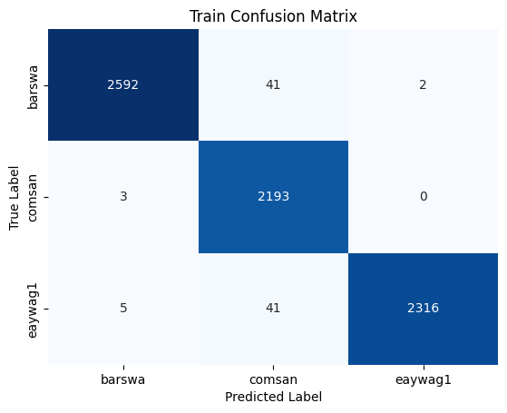
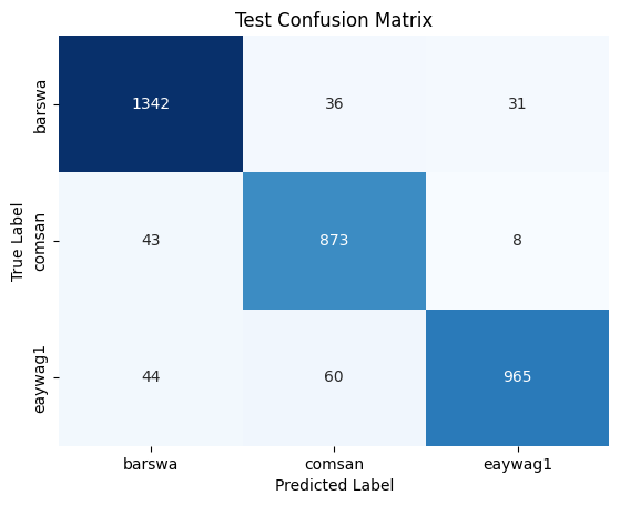
Now that the model is finally performing decently well, it's important to review the confusion matrix and classification reports for the training and validation sets to get a better understanding of which species the model struggles with.
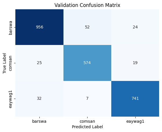
To interpret the confusion matrix, let's take barswa as example. From the validation confusion matrix, we can see that when the true label is barswa, the model mistook barswa for comsan in 67 instances and mistook barswa for eaywag1 in 25 instances. In our EDA performed earlier, we know that barswa had proportionally more poor quality recordings in the training set than the other two species, but the performance on barswa is actually comparable to the other two, this can be seen from the f1 score in the classification report as well. Notabily comsan had lower precision and eaywag1 had lower recall, where as barswa has balanced precision and recall, but the overall f1 score among all three species were comparable.


I further ran comparable models by omitting the continents to evaluate whether the continents contribute to the overall model performance. With continents omitted, the best performing 1D CNN model (with similar architecture as above, with the same hyper-parameters) had the highest validation accuracy of 89%, evidence that including continents as feature in our models does improve the model performance.
To perform hyperparameter tuning on the best performing model (highlighted above), I utilized HyperOpt, a Python library for hyperparameter optimization. Hyperparameters selected for hyperparameter tuning are: learning rate, number of hidden layers, filter size, kernel size, stride size, pooling size, regularization strength, dropout rate, number of nodes in the last fully connected layer, and batch size. The different hyperarameters did not make a notable difference in the model performance, details can be seen in the c.1DCNN_8sec_w_continents_hyperopt.ipynb file.
F2. 2D Convolutional Neural Networks (2D CNN)
Since the 1D CNN model (and prior models) showed 8 seconds framed audios without augmentation with MFCC(20) + RMS(1) + Spectral Centroid(1) + Continents(2) as features had the best performance, I implemented the 2D CNN model with tensorflow functional API architecture with these features.
Compare to 1D CNN models where the filters only move down, the filters in 2D CNN models move in 2 directions: to the right and down. There are two ways of constructing the features for the 2D CNN model:
- use the same features as what was used in the 1D CNN model by concatenating the features so we have features of shape [n_frame, n_features], or
- consider each feature as a different channel, effectively creating features of shape [n_frame, n_features, n_channels]
I decided to go with the second option, below is an illustration of the features using the second option.
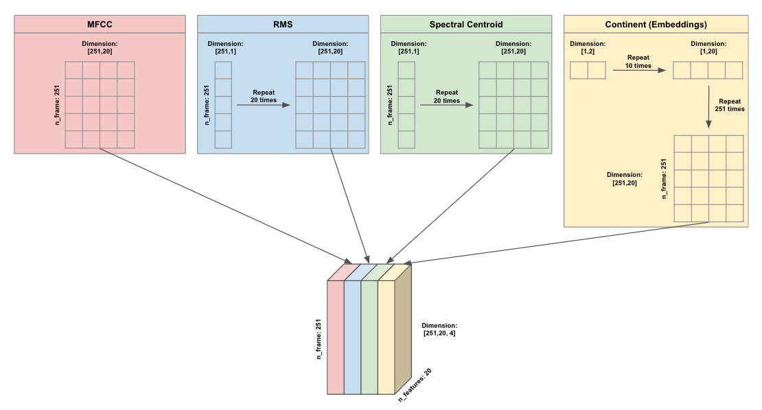
With MFCC as the main feature of shape [n_frames, n_features] = [251, 20], RMS is tiled/repeated 20 times at each time step to match the shape of MFCC, the same was done for Spectral Centroid. Since continents embeddings had shape of [,embedding_dim] = [,2], the continents embeddings were first tiled/repeated 10 times along the features dimension and then repeated 251 times along the time dimension to match the shape of MFCC. After all features have shape [251, 20], they are stacked on top of each other to create a combined 3D features with shape [n_frame, n_features, n_channels] = [251, 20, 4], where the n_channels can be viewed similar to the number of colors in an image classification 2D CNN task.
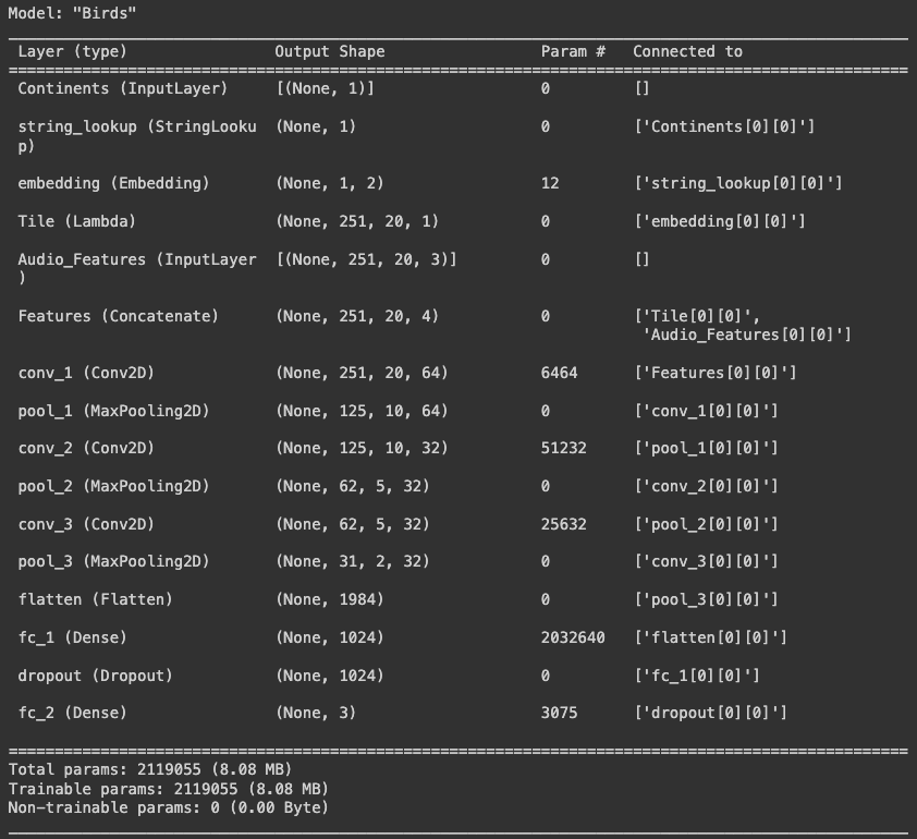
As can be seen in the model summary above, the model consisted of three 2D conv layers (each with kernel_size=(5,5), strides=(1,1), activated with the ReLU activation function, and L2 regularization=0.02, with the first layer having 64 filters and the two following layers having 32 filters each), each layer is followed by a max pooling layer (each with pool_size=(2,2)). The model is then followed by a flattening layer and then a fully connected layer (with units=1024), before being passed to a 50% dropout layer, which finally leads to the output layer. Similar to the 1D CNN model, I also utilized the 'rating' feature to create sample weights to give audio samples with worse ratings less weights during training. L2 regularization and dropout were employed to reduce overfitting, and callback technique was used to call the model back to the epoch with the highest weighted validation accuracy. The model was trained with the Adam optimizer, 0.001 learning rate, and batch size of 32.
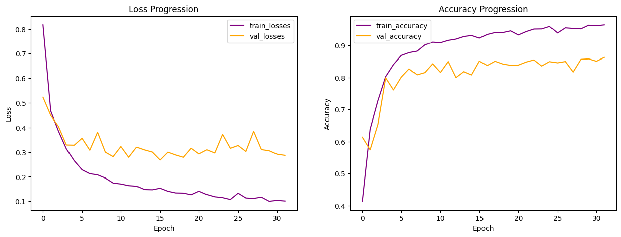
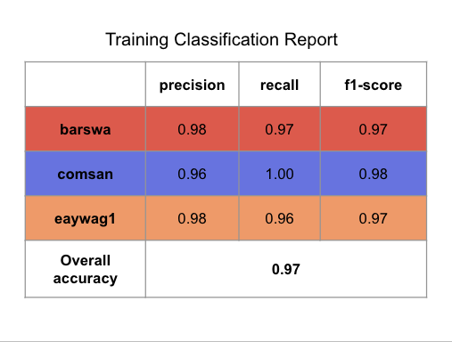
The model reached its highest validation accuracy of 86% at epoch 31, this validation accuracy is slightly lower than that of the best performing 1D CNN model above, but still outperforms any other previously implemented models. The model is also more overfitted than the 1D CNN model above, suggesting stronger regularization or more dropout between the hidden layers might be beneficial. Notably 2D CNN is much more computationally expensive compared to 1D but the performance was not any better, this could be attributed to the fact that the model was not hypertuned and that 2D CNNs are generally better for image classification tasks when we have an audio classification task. The classification reports and confusion matrixes are presented below for completeness sake, but I won't discuss them in detail.
G1. Recurrent Neural Networks - Long short-term memory (LSTM RNN)
Long Short-Term Memory (LSTM) is one of the Recurrent Neural Networks (RNN), developed to solve the vanishing gradient and memoery loss issue with the traditional RNNs. Like RNNs in generally, LSTM are commonly used for sequential data, such as text and audios.
For the LSTM models, I used 8 seconds framed audios without augmentation with audio features only. Similar to what I had done with the previous models, I experimented with different combinations of audio features using the same model architecture and hyperparameters and found that the combination of 20 MFCC + 1 Spectral Centroid had the best performance, as evidenced in the table below.
| Features | Training Accuracy | Validation Accuracy |
|---|---|---|
| MFCC(20) + Chroma(12) | 0.98 | 0.86 |
| MFCC(20) + RMS(1) + Spectral Centroid(1) | 0.99 | 0.89 |
| MFCC(20) + Chroma(12) + RMS(1) + Spectral Centroid(1) | 0.99 | 0.90 |
| MFCC(20) + RMS(1) | 0.98 | 0.91 |
| MFCC(20) + Spectral Centroid(1) | 0.97 | 0.91 |
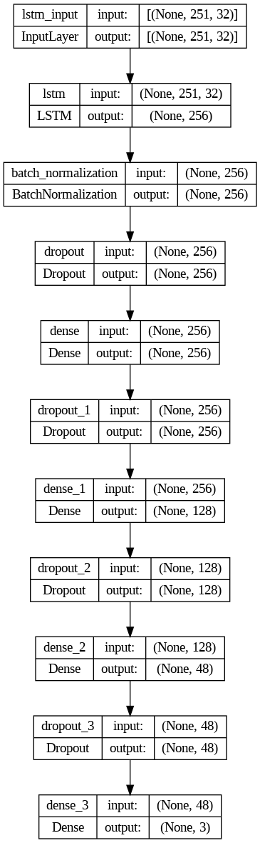
All models were ran with the same architecture: one LSTM layer with 256 nodes, followed by a BatchNormalization layer and a dropout layer with dropout=0.3, followed by three dense layers (each with 256, 128, and 48 nodes respectively, activated with the ReLU activation function, and L2 regularization=0.01) each followed by a dropout layer (dropout=0.3), before being passed to the output layer. Differ from the FFNN and CNNs where the Keras Functional API architecture was used, I used the Keras Sequential modeling for the LSTMs, adhering to the sequential nature of the LSTM model architecture. The 'rating' feature was used to create sample weights to give audio samples with worse ratings less weights during training. L2 regularization and dropout were employed to reduce overfitting, and callback technique was used to call the model back to the epoch with the highest weighted validation accuracy. All models were trained with the Adam optimizer, 0.002 learning rate, and batch size of 64. Note that another teammember experimented on the number of dense layers and the nodes for each layer and the specifications used here is based on the optimal results from that experiment.
A visualization of the model architecture can be seen on the left, this visualization uses 20 MFCC + 12 Chroma as the audio features for each 8 seconds framed audio.
Below is the learning curves from the best performing model (highlighted above). Compared to the learning curves from the CNN models, we observe more prominent zig zags, suggesting the model is still struggling from one epoch to another.
By comparing the confusion matrix and classification reports for the training and validation sets against the best performing 1D CNN model above, we see that the performance between the two models are comparable, with the LSTM model being ever so slightly less overfitted and showing marginally better recall for barswa and comsan than the 1D CNN model.


G2. Recurrent Neural Networks - Gated Recurrent Unit (GRU RNN)
Similar to LSTM, Gated Recurrent Unit (GRU) is also a Recurrent Neural Network (RNN). Differ from LSTM, it employs a gated mechanism and uses fewer parameters. The GRU models were ran using the same features, model archiecture, and hyperparameters as the LSTM models, with the only difference being the LSTM layer was replaced with the GRU layer. Below is a summary of the model results.
| Features | Training Accuracy | Validation Accuracy |
|---|---|---|
| MFCC(20) + Spectral Centroid(1) | 0.98 | 0.91 |
| MFCC(20) + Chroma(12) + RMS(1) + Spectral Centroid(1) | 1.00 | 0.92 |
| MFCC(20) + Chroma(12) | 1.00 | 0.93 |
| MFCC(20) + RMS(1) + Spectral Centroid(1) | 0.99 | 0.93 |
| MFCC(20) + RMS(1) | 0.99 | 0.93 |
The model with 20 MFCC + 1 RMS + 1 Spectral Centroid performed equally well as the model without Spectral Centroid, suggesting the addition of Spectral Centroid did not add substantial value to the model performance, therefore, I will focus on the model without Spectral Centroid for the analysis of the results. This is the best performing model so far, with the validation accuracy at 93%, exceeding the validation accuracy of all previous models.
Compared to the learning curves from the LSTM model, the zig zags are less predominent. And the two learning curves are more closely together with the training curve performing slightly better than the validation curve, suggesting less overfitting and overall better performance than all previous models.
By comparing the confusion matrix and classification reports for the training and validation sets against the best performing 1D CNN model above, we see that the GRU model outperforms the 1D CNN model in almost all metrics for all three species.
H1. Transformer
I did not experiment with using a transformer architecture at the time of the project, a separate project is dedicated to experiments conducted using a vision transformer architecture on the same dataset.
J1. Transfer Learning
A separate project is dedicated to experiments conducted using transfer learning on the same dataset.
INFERENCE
Now that the trainings are completed, it is finally time to run inference on the test data. Given the 1D CNN and the GRU RNN models performed the best amongst all models, I ran inference using the trained weights from these two models.
All notebooks for the inference can be found in the 5.inference folder in the GitHub repo.
A1. Data Preparation
The inference should be run using the same features as was used for training. First, the framed audios were extracted using the a1.inference_8sec.ipynb notebook, where the Framed class method is used. This is the same notebook in the 3.model_prep/c.extract_framed_audios/8sec.ipynb notebook that was used on the training data, note that I changed the class method slightly to accommodate for the test data.
Once the framed audios were extracted, the labels and audio features were extracted using the a2.inference_8_sec_audio_features_not_avgpooled.ipynb notebook by passing in the train_df and test_df to the Extraction class method. This is the same notebook as 3.model_prep/d.extract_feature_labels/8_sec_audio_features_not_avgpooled.ipynb notebook. It is important to pass in both train_df and test_df as the feature normalization scaler should be fit using the training data to prevent data leakage.
Similarly, the non-audio features were extracted using the a3.inference_8_sec_non_audio_features.ipynb notebook by passing in the train_df and test_df to the Extraction class method. This is the same notebook as 3.model_prep/d.extract_feature_labels/8_sec_non_audio_features.ipynb notebook. It is not neccessary to pass in train_df but I still passed in the train_df for convenience sake (so I wouldn't need to make adjustments to the Extraction class).
B1. 1D CNN
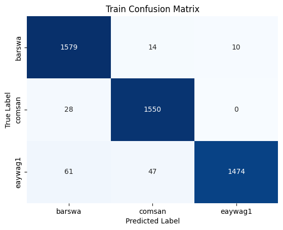
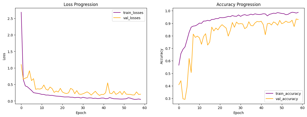
It is common to combine the training and validation set as one combined training set to train the best performing model with the same hypertuned hyperparameters one last time before using the final model for inference, so that is what I did for running the inference as well. I combined the training and validation set to one training dataset, used 20 MFCC, 1 RMS, 1 Spectral Centroid, with continents of embedding size = 2 as the main features with rating as sample weights, using the same hyperparameters as the hypertuned training model to train the model one last time. The model was trained for 35 epochs with no callback. Once the model is done training, I ran inference on the test set using the same features. Below summarized is the resulting classification report and the confusion matrix.
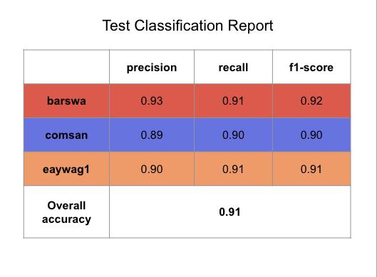

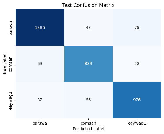
Compared to the original training results, we can see that the model performed slightly better on the test set (compared to the validation set) for barswa and comsan and slightly worse for eaywag1, although the difference is negligible. The test result is comparable to that of the validation result, suggesting the model is generalizing reasonabily well to the unseen test set. The overall test accuracy of 91% is also reasonabily high, as compared to the baseline.
C1. GRU RNN
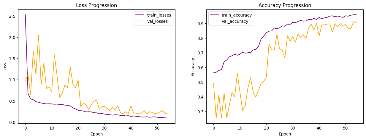
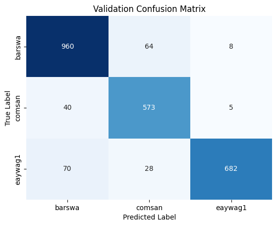
Similar to what I did for inference on 1D CNN, I combined the training and validation set to one training dataset to train the model one last time before running inference using the GRU RNN model.Following the best performing GRU RNN training model, I used 20 MFCC + 1 RMS without continents as the main features with rating as sample weights, using the same hyperparameters as the hypertuned training model. The model was trained for 58 epochs with no callback. Once the model is done training, I ran inference on the test set using the same features. Below summarized is the resulting classification report and the confusion matrix.

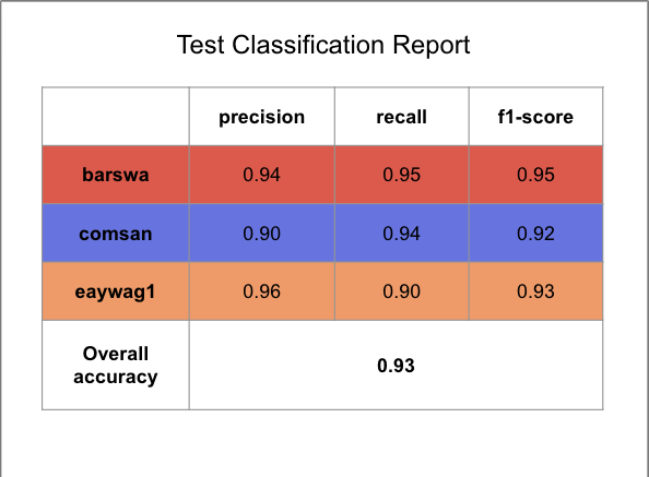
The result is similar to that of the 1D CNN inference results, but with slightly higher overall accuracy and better performance across all three species. This is expected as RNNs are generally better suited for sequence processing tasks, whereas CNNs are generally better suited for image classification tasks. Audios, a form of digital signal, are sequential in nature. Although, by converting audio to spectrograms, therefore converting a digital signal processing task to a computer task seem to also yield promissing results. It is notable that CNNs are faster than RNNs, so perhaps the slight reduction in performance is affordable considering the potential in efficieny gain, although more thorough analysis should be performed to draw meaningful conclusions. The overall test accuracy of 93% is also reasonabily high, as compared to the baseline and as compared to all other models experimented.
LIMITATIONS
The biggest limitation of the project is that I only selected three of the most common bird species for the classification task, therefore, the models are not robust towards other bird species. I also did not perform ablation study for all models experimented, therefore, the model performance could be further improved if more comprehensive hypertuning were performed.
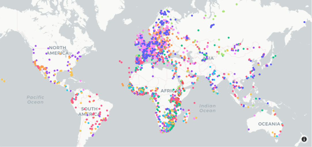
Another notable limitation pertains to the fairness of the original dataset. The map view (generated by another teammember) below shows the geographical distribution of the samples, with each dot representing one sample and each color corresponding to a specific species. We can see that majority of the samples are sourced from Europe, closely followed by South Afric, while birds from other regions of the world (Americas, Oceania, Asia) are under-represented. We could improve fairness by adjusting the data gathering process or sample weighting scheme to create more generalizable bird song classification models for birds from all over the world.
GITHUB
Please see my GitHub for the code for the project.